Indice
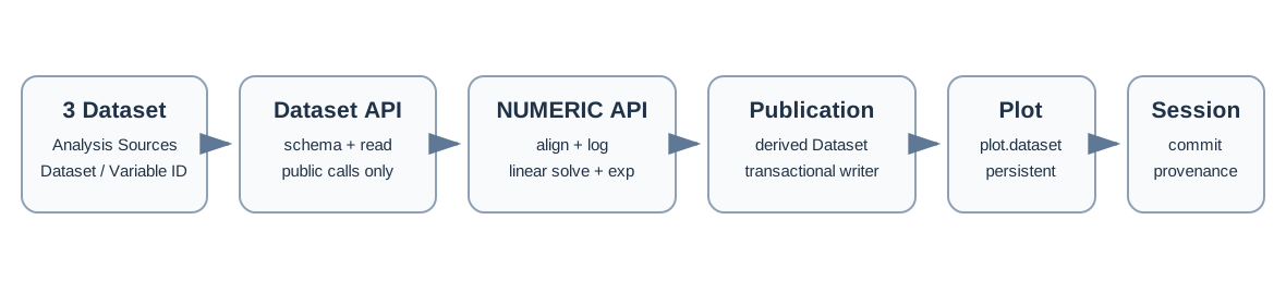
Il tutorial costruisce uno script di ricerca GNU Octave che prende tre scariche RC campionate in punti temporali differenti, le legge come Dataset canonici GX-TXT, le allinea attraverso le API numeriche, stima la costante di tempo tau, pubblica un Dataset derivato e crea un grafico persistente con plot.dataset.
1. Obiettivo, modello e file dell'esercizio
1.1 Che cosa costruiamo
several RC discharge Datasets
        ↓
GX-TXT Analysis Source aliases
        ↓
Canonical Dataset API
        ↓
NUMERIC_API interpolation/alignment
        ↓
multisource consensus curve
        ↓
NUMERIC_API fit
        ↓
derived GX-TXT Dataset
        ↓
plot.dataset 2D graph
Il modello fisico è la scarica RC ideale a offset finale nullo:
V(t) = V0 * exp(-t/tau)
tau = R*C
Prendendo il logaritmo naturale:
ln(V) = ln(V0) - t/tausi ottiene un problema lineare in ln(V). Questo permette di introdurre allineamento, algebra lineare, pubblicazione e plotting senza richiedere ancora callback di fit non lineare.
1.2 File forniti
Ogni CSV contiene:
time_s
voltage_V
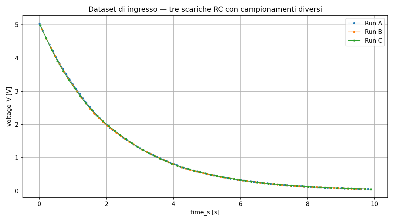
I tre Dataset hanno posizioni temporali leggermente diverse. È una caratteristica voluta: prima della media devono essere allineati su una griglia comune.
1.3 Semplificazione del modello
Il tutorial assume:
final discharge voltage = 0Il modello è quindi V0 * exp(-t/tau). Un modello con offset finale, per esempio V_offset + A * exp(-t/tau), richiede un fit non lineare vero e proprio.
2. Preparare Session, Workspace e Script Library
2.1 Importare i tre CSV
Crea o apri una Session pulita e importa i tre file con Generic CSV. Usa Dataset ID riconoscibili, per esempio:
rc_run_A
rc_run_B
rc_run_C
Verifica che ciascun Dataset contenga le variabili numeriche time_s e voltage_V.
2.2 Attivare Octave Script e aprire il Viewer
Abilita il modulo:
Octave Script
Module ID: analysis.octave_script
Apri:
Viewers
→ Octave Script Workspace
→ New
Assegna al documento un nome come RC multisource discharge fit. Importa rc_discharge_multisource_fit.m oppure copiane il contenuto nel Workspace e salva il documento.
2.3 Workspace e script eseguibile non sono lo stesso oggetto
Il documento del Workspace è una risorsa interattiva persistente della Session. Il runner riproducibile esegue invece uno script registrato nella Script Library.
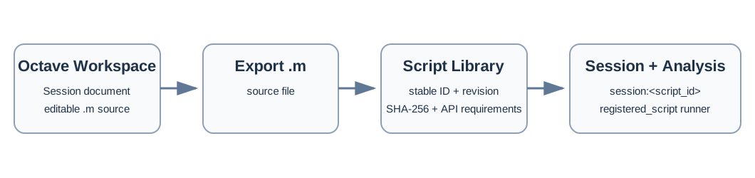
Octave Script Workspace
        ↓
Export .m
        ↓
Script Library
        ↓
user:<script_id>
        ↓
Assign to Session
        ↓
session:<script_id>
        ↓
normal Analysis runner
2.4 Registrare lo script
Esporta dal Viewer il file rc_discharge_multisource_fit.m, apri Script Library... e importalo. Metadati consigliati:
Stable ID:    tutorial.rc_discharge_fit
Display name: RC Multisource Discharge Fit
Version:      1.0.0
Language:     Octave
Dichiara le API pubbliche richieste:
CANONICAL_DATASET_API_v2@2;
DATASET_VARIABLE_SCHEMA_API_v3@3;
NUMERIC_API_v1@1:math.numeric;
DATASET_PUBLICATION_API_v2@2;
PLOT_DATASET_API_v3@3:plot.dataset+plotspec;
SESSION_PERSISTENCE_API_v1@1
GX-TXT verifica questi requisiti prima dell'avvio dello script. Se manca un servizio necessario, il run si interrompe prima di eseguire il calcolo.
2.5 Assegnare lo script alla Session
Da Script Library scegli Assign to Session. Il riferimento diventa, per esempio:
session:tutorial.rc_discharge_fitNella configurazione di Octave Script scegli:
Source mode = registered_script
Script      = session:tutorial.rc_discharge_fit
3. Collegare più Dataset e leggerli attraverso le API pubbliche
3.1 Analysis Sources multisorgente
Seleziona un Dataset come primary e aggiungi gli altri due con + Add source. La mappa può risultare, per esempio:
primary     → rc_run_A
additional  → rc_run_B
additional  → rc_run_C
Lo script non dipende dai nomi dinamici assegnati agli alias. Scopre tutti gli ingressi popolati partendo dal context.
3.2 gxtxt_context()
ctx = gxtxt_context();
aliases = fieldnames(ctx.inputs);
Per ogni alias popolato lo script recupera il relativo dataset_id. Non bisogna codificare nello script nomi dinamici come source2.
3.3 Dataset ID e Variable ID, non percorsi
Dopo l'importazione lo script non apre direttamente rc_discharge_run_A.csv. L'identità scientifica utilizzata dal workflow è:
Dataset ID
Variable ID
Per ogni Dataset lo schema viene letto con:
schema = gxtxt_api_call(
    'DATASET_VARIABLE_SCHEMA_API_v3',
    'list',
    {dataset_id});
Il codice cerca le variabili canoniche time_s e voltage_V e ne conserva gli ID stabili.
3.4 Lettura dei dati
Prima si legge la descrizione:
meta = gxtxt_api_call(
    'CANONICAL_DATASET_API_v2',
    'describe',
    {dataset_id});
poi l'intervallo di righe necessario:
block = gxtxt_api_call(
    'CANONICAL_DATASET_API_v2',
    'read_range',
    {dataset_id, {time_id, voltage_id}, 0, meta.row_count});
I valori sono restituiti sotto i rispettivi Variable ID. Nessun file privato del Dataset viene aperto direttamente.
3.5 Ordinamento e intervallo temporale comune
L'allineamento richiede coordinate strettamente crescenti:
[t, order] = sort(t);
v = v(order);
Il tutorial rifiuta coordinate duplicate o non crescenti. L'intervallo comune viene scelto come intersezione di tutte le acquisizioni:
common_start = max(all source starts)
common_stop  = min(all source stops)
time_common  = linspace(common_start, common_stop, 200)'
Usare l'intersezione evita di introdurre extrapolazione implicita.
4. Allineare le curve e costruire la curva di consenso
4.1 Chiamare NUMERIC_API_v1
Uno script registrato usa gxtxt_api_call(...) per raggiungere i servizi pubblici. Per allineare una famiglia di curve campionate si usa l'operazione:
NUMERIC_API_v1 / foundation
family / align
Il risultato è una matrice con una colonna per ogni sorgente e una riga per ogni coordinata della griglia comune.
4.2 Nodi tipizzati del bridge
Il bridge scientifico trasporta gli oggetti matematici con nodi tipizzati. L'helper numeric_array_node(values) costruisce un nodo con:
kind  = array
shape = [N,1]
real  = values
Una famiglia di curve viene rappresentata come kind = cell contenente i nodi array. Questa forma consente allo script di usare il servizio numerico pubblico senza dipendere da file di implementazione Octave privati.
4.3 Chiamata di allineamento
aligned = gxtxt_api_call(
    'NUMERIC_API_v1',
    'foundation',
    {'family', 'align',
     time_family,
     voltage_family,
     target_node,
     empty_options});

voltage_aligned = aligned.value_real;
Con tre sorgenti:
column 1 = interpolated run A
column 2 = interpolated run B
column 3 = interpolated run C
4.4 Curva media
voltage_mean = mean(voltage_aligned, 2);La media costituisce la curva di consenso usata per il primo fit. In analisi più avanzate si possono aggiungere deviazione standard, intervalli di confidenza, pesi delle sorgenti e diagnostica degli outlier.
5. Stimare V0 e tau
5.1 Linearizzazione
Per il modello:
V(t) = V0 * exp(-t/tau)si usa:
ln(V) = ln(V0) - t/tauLo script mantiene i soli valori positivi e calcola il logaritmo con l'operazione pubblica:
log_result = gxtxt_api_call(
    'NUMERIC_API_v1',
    'array_unary',
    {'log', log_operand});
5.2 Sistema lineare ai minimi quadrati
La matrice di progetto è:
[1 t]e il problema è:
ln(V) = beta(1) + beta(2)*tLa soluzione viene richiesta a NUMERIC_API_v1:
fit_result = gxtxt_api_call(
    'NUMERIC_API_v1',
    'linear_matrix',
    {'solve', matrix_A, matrix_b});

beta = fit_result.value_real(:);
5.3 Recuperare i parametri fisici
log_V0 = beta(1);
slope = beta(2);

V0_fit = exp(log_V0);
tau_fit = -1 / slope;
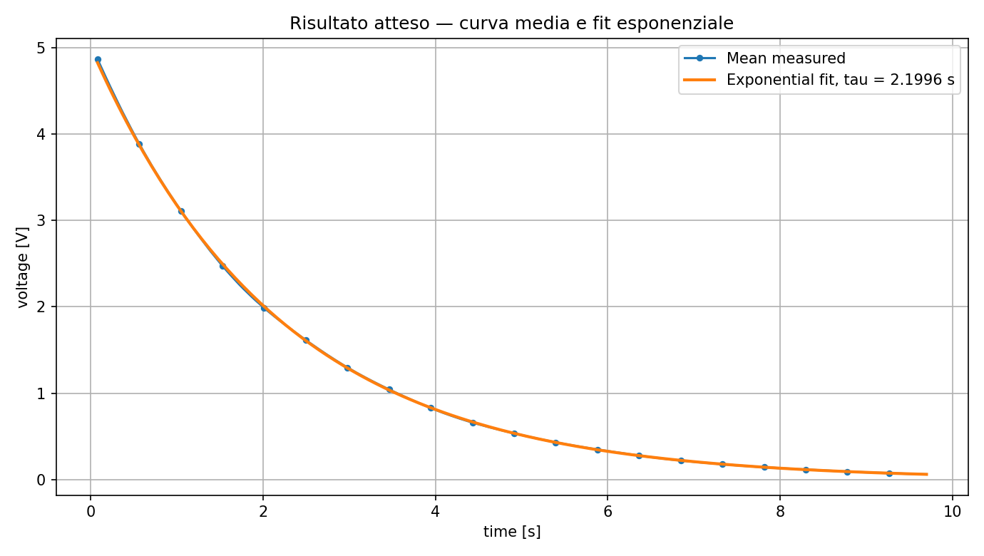
Una scarica RC valida deve fornire slope < 0 e tau > 0. Con i file forniti il risultato atteso è circa:
tau ≈ 2.19961 s
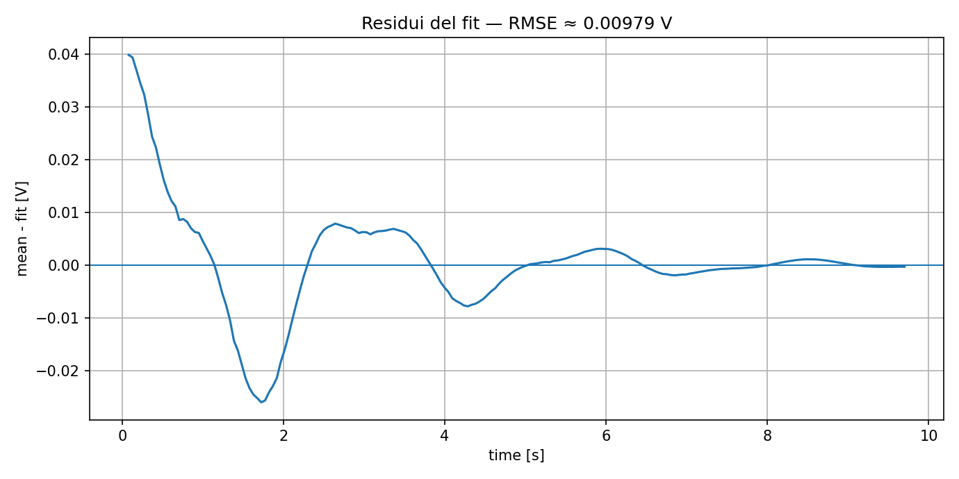
RMSE ≈ 0.009793 V
5.4 Generare la curva fitted
Lo script dimostra le operazioni pubbliche multiply, add ed exp:
slope * t
    ↓
+ log(V0)
    ↓
exp(...)
    ↓
V_fit(t)
A questo punto in memoria sono disponibili time_common, voltage_mean, voltage_fit, residual, oltre a V0_fit, tau_fit e RMSE.
6. Pubblicare il Dataset derivato
6.1 Definizione del risultato
Il Dataset derivato usa l'ID stabile:
tutorial.rc_discharge_fite contiene:
v_time
v_mean
v_fit
v_residual
6.2 Pubblicazione transazionale
La sequenza è:
begin
→ declare dimension
→ declare variables
→ write values
→ finalize
In caso di errore prima della finalizzazione viene eseguito abort. In questo modo un Dataset parzialmente scritto non può comparire come risultato valido.
writer = gxtxt_api_call(
    'DATASET_PUBLICATION_API_v2',
    'begin',
    {definition});
6.3 Dimensione e schema delle variabili
gxtxt_api_call(
    'DATASET_PUBLICATION_API_v2',
    'declare_dimension',
    {writer, 'row', numel(time_common), struct()});
La variabile tempo è una coordinata indipendente; le curve di tensione sono dati misurati o derivati con l'unità ereditata dai Dataset sorgente. Il risultato mantiene quindi uno schema scientifico reale e non è una tabella anonima.
6.4 Scrittura, finalizzazione e replace_owned
Dopo avere scritto tutte le variabili:
published = gxtxt_api_call(
    'DATASET_PUBLICATION_API_v2',
    'finalize',
    {writer});
replace_owned = true permette allo stesso script di aggiornare il proprio Dataset stabile nelle esecuzioni successive invece di generare un nuovo ID ogni volta.
7. Creare il grafico persistente e salvare lo stato
7.1 PlotSpec e Series
Lo script non usa figure() o plot() privati. Richiede un normale PlotSpec:
plot_spec = gxtxt_api_call(
    'PLOT_DATASET_API_v3',
    'new_spec',
    {'plot.dataset.xy',
     'RC discharge: multisource mean and exponential fit'});
Le due Series sono:
Mean measured
X = v_time
Y = v_mean
kind = line_marker

Exponential fit
X = v_time
Y = v_fit
kind = line
Entrambe fanno riferimento al Dataset tutorial.rc_discharge_fit.
7.2 upsert_plot e render
plot_ref = gxtxt_api_call(
    'PLOT_DATASET_API_v3',
    'upsert_plot',
    {'tutorial_rc_discharge_fit', plot_spec});

gxtxt_api_call(
    'PLOT_DATASET_API_v3',
    'render',
    {plot_ref});
upsert_plot crea il plot alla prima esecuzione e aggiorna lo stesso plot persistente nelle esecuzioni successive. Il risultato partecipa ai normali controlli GX-TXT: Series, assi, griglia, legenda, layout, Variant e rerender.
7.3 Commit della Session
gxtxt_api_call(
    'SESSION_PERSISTENCE_API_v1',
    'commit',
    {});
Il commit rende persistente lo stato gestito dal framework creato dallo script. Non è necessario e non è corretto modificare manualmente manifest.ini.
7.4 Report del run
Lo script salva anche rc_fit_report.txt nella directory di output del run con numero di sorgenti, intervallo comune, numero di punti, V0, tau, RMSE e Dataset pubblicato. Il runner conserva inoltre sorgente eseguito, report standard, provenance e SHA-256.
8. Eseguire, verificare e modificare l'esempio
8.1 Esecuzione
- verifica che lo script della Session sia selezionato;
- verifica che i tre Dataset RC siano presenti nelle Analysis Sources;
- esegui Run / recalculate;
- avvia
Octave Script.
L'output deve contenere indicazioni equivalenti a:
Input Datasets: 3
Fit result: V0 = about 5 V, tau = about 2.2 s
Published Dataset: tutorial.rc_discharge_fit
PASS RC tutorial ...
8.2 Controllare Dataset e grafico
Nel Dataset tutorial.rc_discharge_fit devono essere disponibili v_time, v_mean, v_fit e v_residual. Il grafico deve mostrare Mean measured e Exponential fit. Le modifiche ordinarie di presentazione possono essere effettuate con i normali controlli di plot.dataset senza cambiare lo script.
8.3 Limite del fit log-lineare
Il logaritmo modifica il modello dell'errore. Se il rumore di tensione è approssimativamente additivo in volt, i minimi quadrati nello spazio logaritmico non sono equivalenti a un fit non lineare ai minimi quadrati nello spazio delle tensioni. Per i dati didattici forniti la semplificazione è adeguata; per misure reali va scelto il modello statistico e il peso scientificamente appropriati.
8.4 Perché non viene usato nonlinear_fit
Il binding Octave diretto di NUMERIC_API_v1 può supportare fit non lineari basati su callback, ma il generic Script Bridge non serializza function handle Octave eseguibili. Uno script del Viewer non deve quindi aspettarsi che una callback locale attraversi il bridge come avviene in un modulo con binding diretto.
8.5 Modifiche utili
Densità della griglia comune. Cambia:
common_count = 200;in 100 oppure 400 e riesegui. Dataset e plot vengono aggiornati attraverso gli stessi ID stabili.
Dispersione fra sorgenti. Dopo la media aggiungi:
voltage_std = std(voltage_aligned, 0, 2);e pubblica v_std come nuova variabile.
Capacità da una resistenza nota. Se R è un vero input sperimentale:
C = tau / RCon R = 10 kΩ e tau ≈ 2.2 s si ottiene C ≈ 220 µF.
8.6 Errori comuni
| Errore | Approccio corretto |
|---|---|
Codificare ctx.inputs.source2 | Iterare fieldnames(ctx.inputs) e usare tutti gli ingressi popolati. |
| Aprire direttamente il CSV originale | Usare Dataset ID, Variable ID e Canonical Dataset API. |
| Supporre campionamenti identici | Allineare prima le curve su una griglia comune. |
| Extrapolare senza dichiararlo | Usare l'intervallo di sovrapposizione oppure definire esplicitamente una politica di extrapolazione. |
Applicare log a tensioni non positive | Verificare V > 0 prima della linearizzazione. |
Concludere con figure; plot(...) | Pubblicare il Dataset e creare il grafico tramite PLOT_DATASET_API_v3. |
8.7 Separazione delle responsabilità
Lo script possiede:
scientific question
algorithm
choice of model
choice of derived Dataset
GX-TXT possiede:
Dataset identity
source selection
API discovery
numerical service boundary
Dataset publication transaction
plot infrastructure
Session persistence
execution provenance
Questa separazione consente allo script di ricerca di evolvere successivamente in un modulo Analysis dedicato senza cambiare il modello scientifico di base.
8.8 Prossimo esercizio
Un'estensione naturale consiste nel pubblicare v_std, costruire le variabili inferiore/superiore di incertezza, aggiungere una uncertainty band in plot.dataset e creare un secondo grafico dei residui.
9. Sorgente completo
Il file eseguibile completo è disponibile per il download. Puoi anche consultarlo qui per confrontarlo con i passaggi del tutorial.
Mostra rc_discharge_multisource_fit.m
% GX-TXT first Octave Script Workspace scientific workflow.
% Multisource RC discharge alignment, exponential fit, Dataset publication,
% and persistent 2D Plot Dataset graph.
%
% SPDX-License-Identifier: GPL-3.0-or-later

% -------------------------------------------------------------------------
% 1. Inspect the GX-TXT script execution context.
% -------------------------------------------------------------------------
ctx = gxtxt_context();

fprintf('GX-TXT script: %s\n', ctx.script_name);
fprintf('Run ID: %s\n', ctx.run_id);

% This tutorial requires at least two populated Analysis Sources.
if (!isfield(ctx, 'inputs') || !isstruct(ctx.inputs))
  error('RC tutorial: GX-TXT did not provide Analysis Source inputs.');
endif

aliases = fieldnames(ctx.inputs);
source_ids = {};
for k = 1:numel(aliases)
  item = ctx.inputs.(aliases{k});
  if (isstruct(item) && isfield(item, 'dataset_id') && !isempty(item.dataset_id))
    source_ids{end+1} = item.dataset_id;
  endif
endfor

source_ids = unique(source_ids, 'stable');

if (numel(source_ids) < 2)
  error('RC tutorial: select at least two Dataset sources in Analysis.');
endif

fprintf('Input Datasets: %d\n', numel(source_ids));

% -------------------------------------------------------------------------
% 2. Require the public GX-TXT APIs used by the script.
% -------------------------------------------------------------------------
gxtxt_api_require({
  'CANONICAL_DATASET_API_v2@2',
  'DATASET_VARIABLE_SCHEMA_API_v3@3',
  'NUMERIC_API_v1@1:math.numeric',
  'DATASET_PUBLICATION_API_v2@2',
  'PLOT_DATASET_API_v3@3:plot.dataset+plotspec',
  'SESSION_PERSISTENCE_API_v1@1'
});

% -------------------------------------------------------------------------
% 3. Read every source Dataset through public Dataset APIs.
%
% The tutorial expects canonical variables named:
%   time_s
%   voltage_V
% -------------------------------------------------------------------------
time_cells = cell(1, numel(source_ids));
voltage_cells = cell(1, numel(source_ids));
source_variable_ids = {};
time_unit = '';
voltage_unit = '';

for s = 1:numel(source_ids)
  dataset_id = source_ids{s};

  schema = gxtxt_api_call(
      'DATASET_VARIABLE_SCHEMA_API_v3',
      'list',
      {dataset_id});

  time_id = find_variable_id(schema, 'time_s');
  voltage_id = find_variable_id(schema, 'voltage_V');

  if (isempty(time_id) || isempty(voltage_id))
    error('RC tutorial: Dataset %s must contain time_s and voltage_V.', dataset_id);
  endif

  meta = gxtxt_api_call(
      'CANONICAL_DATASET_API_v2',
      'describe',
      {dataset_id});

  block = gxtxt_api_call(
      'CANONICAL_DATASET_API_v2',
      'read_range',
      {dataset_id, {time_id, voltage_id}, 0, meta.row_count});

  t = block.(time_id).values(:);
  v = block.(voltage_id).values(:);

  good = isfinite(t) & isfinite(v);
  t = t(good);
  v = v(good);

  if (numel(t) < 5)
    error('RC tutorial: Dataset %s contains too few finite points.', dataset_id);
  endif

  % NUMERIC_API family alignment requires strictly increasing coordinates.
  [t, order] = sort(t);
  v = v(order);

  if (any(diff(t) <= 0))
    error('RC tutorial: Dataset %s contains duplicate/non-increasing time values.', dataset_id);
  endif

  if (any(v <= 0))
    error('RC tutorial: voltage must remain positive for the log-linear RC fit.');
  endif

  time_cells{s} = t;
  voltage_cells{s} = v;

  tdesc = variable_by_id(schema, time_id);
  vdesc = variable_by_id(schema, voltage_id);

  if (isempty(time_unit)), time_unit = tdesc.unit; endif
  if (isempty(voltage_unit)), voltage_unit = vdesc.unit; endif

  source_variable_ids{end+1} = time_id;
  source_variable_ids{end+1} = voltage_id;

  fprintf('  %s: rows=%d range=[%.6g, %.6g]\n', ...
          dataset_id, numel(t), t(1), t(end));
endfor

source_variable_ids = unique(source_variable_ids, 'stable');

% -------------------------------------------------------------------------
% 4. Build one common time grid.
%
% We use only the overlap shared by every source, so interpolation never
% requires extrapolation.
% -------------------------------------------------------------------------
common_start = -Inf;
common_stop = Inf;

for s = 1:numel(time_cells)
  common_start = max(common_start, time_cells{s}(1));
  common_stop = min(common_stop, time_cells{s}(end));
endfor

if (!(common_stop > common_start))
  error('RC tutorial: the selected sources have no common time interval.');
endif

common_count = 200;
time_common = linspace(common_start, common_stop, common_count).';

% -------------------------------------------------------------------------
% 5. Interpolate all source curves through NUMERIC_API_v1.
%
% The Script Bridge exposes the mathematical-foundation family alignment
% operation.  It accepts typed transport nodes and returns one matrix column
% per source curve.
% -------------------------------------------------------------------------
empty_node = struct('kind', 'empty');
empty_options = struct('kind', 'struct', 'fields', struct());

time_nodes = cell(1, numel(time_cells));
voltage_nodes = cell(1, numel(voltage_cells));

for s = 1:numel(time_cells)
  time_nodes{s} = numeric_array_node(time_cells{s});
  voltage_nodes{s} = numeric_array_node(voltage_cells{s});
endfor

time_family = struct('kind', 'cell', 'items', {time_nodes});
voltage_family = struct('kind', 'cell', 'items', {voltage_nodes});
target_node = numeric_array_node(time_common);

aligned = gxtxt_api_call(
    'NUMERIC_API_v1',
    'foundation',
    {'family', 'align', time_family, voltage_family, target_node, empty_options});

voltage_aligned = aligned.value_real;

if (rows(voltage_aligned) != numel(time_common) || ...
    columns(voltage_aligned) != numel(source_ids))
  error('RC tutorial: unexpected aligned matrix shape.');
endif

voltage_mean = mean(voltage_aligned, 2);

% -------------------------------------------------------------------------
% 6. Fit the zero-offset RC discharge model:
%
%      V(t) = V0 * exp(-t/tau)
%
% Taking the logarithm:
%
%      ln(V) = ln(V0) - t/tau
%
% The logarithm is obtained through NUMERIC_API array_unary, and the
% overdetermined linear system is solved through NUMERIC_API linear_matrix.
% -------------------------------------------------------------------------
positive = isfinite(voltage_mean) & voltage_mean > 0;
t_fit = time_common(positive);
v_fit_input = voltage_mean(positive);

if (numel(t_fit) < 3)
  error('RC tutorial: too few positive consensus points for fitting.');
endif

log_operand = struct('kind', 'vector', 'value', v_fit_input);
log_result = gxtxt_api_call(
    'NUMERIC_API_v1',
    'array_unary',
    {'log', log_operand});
log_voltage = log_result.values(:);

design = [ones(numel(t_fit), 1), t_fit];
rhs = log_voltage;

matrix_A = struct('real', design);
matrix_b = struct('real', rhs);

fit_result = gxtxt_api_call(
    'NUMERIC_API_v1',
    'linear_matrix',
    {'solve', matrix_A, matrix_b});

beta = fit_result.value_real(:);

if (numel(beta) != 2)
  error('RC tutorial: unexpected fit coefficient count.');
endif

log_V0 = beta(1);
slope = beta(2);

if (!(slope < 0))
  error('RC tutorial: fitted slope is not negative; this is not an RC discharge.');
endif

V0_fit = exp(log_V0);
tau_fit = -1 / slope;

fprintf('Fit result: V0 = %.8g V, tau = %.8g s\n', V0_fit, tau_fit);

% -------------------------------------------------------------------------
% 7. Generate the fitted curve through NUMERIC_API array operations.
% -------------------------------------------------------------------------
t_operand = struct('kind', 'vector', 'value', time_common);
slope_operand = struct('kind', 'scalar', 'value', slope);
offset_operand = struct('kind', 'scalar', 'value', log_V0);

scaled_t = gxtxt_api_call(
    'NUMERIC_API_v1',
    'array_binary',
    {'multiply', t_operand, slope_operand});

affine = gxtxt_api_call(
    'NUMERIC_API_v1',
    'array_binary',
    {'add', struct('kind','vector','value',scaled_t.values), offset_operand});

exp_result = gxtxt_api_call(
    'NUMERIC_API_v1',
    'array_unary',
    {'exp', struct('kind','vector','value',affine.values)});

voltage_fit = exp_result.values(:);
residual = voltage_mean - voltage_fit;

rmse = sqrt(mean(residual.^2));

% -------------------------------------------------------------------------
% 8. Publish the derived result as a canonical GX-TXT Dataset.
% -------------------------------------------------------------------------
result_dataset_id = 'tutorial.rc_discharge_fit';

definition = struct();
definition.dataset_id = result_dataset_id;
definition.contract = 'table.generic';
definition.storage = 'auto';
definition.replace_owned = true;
definition.producer_version = '1.0.0';
definition.source_dataset_ids = source_ids;
definition.source_variable_ids = source_variable_ids;
definition.notes = sprintf('Multisource RC discharge fit: tau=%.9g s, V0=%.9g V', ...
                           tau_fit, V0_fit);

writer = gxtxt_api_call(
    'DATASET_PUBLICATION_API_v2',
    'begin',
    {definition});

try
  gxtxt_api_call(
      'DATASET_PUBLICATION_API_v2',
      'declare_dimension',
      {writer, 'row', numel(time_common), struct()});

  time_schema = struct(
      'dtype', 'float64',
      'rank', 1,
      'dimension_ids', 'row',
      'coordinate_role', 'coordinate',
      'semantic_role', 'independent',
      'unit', time_unit);

  mean_schema = struct(
      'dtype', 'float64',
      'rank', 1,
      'dimension_ids', 'row',
      'coordinate_role', 'data',
      'semantic_role', 'measured',
      'unit', voltage_unit);

  fit_schema = struct(
      'dtype', 'float64',
      'rank', 1,
      'dimension_ids', 'row',
      'coordinate_role', 'data',
      'semantic_role', 'derived',
      'unit', voltage_unit);

  residual_schema = fit_schema;

  gxtxt_api_call(
      'DATASET_PUBLICATION_API_v2',
      'declare_variable',
      {writer, 'v_time', time_schema});

  gxtxt_api_call(
      'DATASET_PUBLICATION_API_v2',
      'declare_variable',
      {writer, 'v_mean', mean_schema});

  gxtxt_api_call(
      'DATASET_PUBLICATION_API_v2',
      'declare_variable',
      {writer, 'v_fit', fit_schema});

  gxtxt_api_call(
      'DATASET_PUBLICATION_API_v2',
      'declare_variable',
      {writer, 'v_residual', residual_schema});

  gxtxt_api_call(
      'DATASET_PUBLICATION_API_v2',
      'write_variable',
      {writer, 'v_time', time_common, numel(time_common)});

  gxtxt_api_call(
      'DATASET_PUBLICATION_API_v2',
      'write_variable',
      {writer, 'v_mean', voltage_mean, numel(voltage_mean)});

  gxtxt_api_call(
      'DATASET_PUBLICATION_API_v2',
      'write_variable',
      {writer, 'v_fit', voltage_fit, numel(voltage_fit)});

  gxtxt_api_call(
      'DATASET_PUBLICATION_API_v2',
      'write_variable',
      {writer, 'v_residual', residual, numel(residual)});

  published = gxtxt_api_call(
      'DATASET_PUBLICATION_API_v2',
      'finalize',
      {writer});

  writer = '';
catch err
  if (!isempty(writer))
    gxtxt_api_call(
        'DATASET_PUBLICATION_API_v2',
        'abort',
        {writer});
  endif
  rethrow(err);
end

fprintf('Published Dataset: %s\n', published.dataset_id);

% -------------------------------------------------------------------------
% 9. Create one simple persistent GX-TXT 2D graph.
% -------------------------------------------------------------------------
plot_spec = gxtxt_api_call(
    'PLOT_DATASET_API_v3',
    'new_spec',
    {'plot.dataset.xy', 'RC discharge: multisource mean and exponential fit'});

panel = plot_spec.panels{1};

measured_series = struct(
    'id', 'mean_measured',
    'dataset_id', result_dataset_id,
    'x_variable_id', 'v_time',
    'y_variable_id', 'v_mean',
    'axis', 'left',
    'kind', 'line_marker',
    'label', 'Mean measured');

fit_series = struct(
    'id', 'exponential_fit',
    'dataset_id', result_dataset_id,
    'x_variable_id', 'v_time',
    'y_variable_id', 'v_fit',
    'axis', 'left',
    'kind', 'line',
    'label', sprintf('Exponential fit, tau = %.4g s', tau_fit));

panel.series = {measured_series, fit_series};
plot_spec.panels = {panel};

gxtxt_api_call(
    'PLOT_DATASET_API_v3',
    'validate_spec',
    {plot_spec});

plot_ref = gxtxt_api_call(
    'PLOT_DATASET_API_v3',
    'upsert_plot',
    {'tutorial_rc_discharge_fit', plot_spec});

gxtxt_api_call(
    'PLOT_DATASET_API_v3',
    'render',
    {plot_ref});

% -------------------------------------------------------------------------
% 10. Save a small human-readable report in this script run directory.
% -------------------------------------------------------------------------
report_path = fullfile(ctx.output_dir, 'rc_fit_report.txt');
fid = fopen(report_path, 'w');
if (fid >= 0)
  fprintf(fid, 'GX-TXT RC discharge tutorial\n');
  fprintf(fid, '============================\n\n');
  fprintf(fid, 'Input Dataset count: %d\n', numel(source_ids));
  fprintf(fid, 'Common interval: %.9g .. %.9g %s\n', ...
          common_start, common_stop, time_unit);
  fprintf(fid, 'Common grid points: %d\n', numel(time_common));
  fprintf(fid, 'Fitted V0: %.12g %s\n', V0_fit, voltage_unit);
  fprintf(fid, 'Fitted tau: %.12g %s\n', tau_fit, time_unit);
  fprintf(fid, 'Consensus RMSE: %.12g %s\n', rmse, voltage_unit);
  fprintf(fid, 'Published Dataset: %s\n', result_dataset_id);
  fclose(fid);
endif

% Persist the newly published Dataset and persistent Plot Dataset Variant.
gxtxt_api_call(
    'SESSION_PERSISTENCE_API_v1',
    'commit',
    {});

fprintf('PASS RC tutorial: Dataset=%s tau=%.8g %s variant=%s\n', ...
        result_dataset_id, tau_fit, time_unit, plot_ref.variant_id);

% =========================================================================
% Local helper functions
% =========================================================================

function variable_id = find_variable_id(schema, canonical_name)
  variable_id = '';
  for i = 1:numel(schema)
    item = schema{i};
    if (isstruct(item) && isfield(item, 'canonical') && ...
        strcmp(item.canonical, canonical_name))
      variable_id = item.variable_id;
      return;
    endif
  endfor
endfunction

function item = variable_by_id(schema, variable_id)
  item = struct();
  for i = 1:numel(schema)
    candidate = schema{i};
    if (isstruct(candidate) && isfield(candidate, 'variable_id') && ...
        strcmp(candidate.variable_id, variable_id))
      item = candidate;
      return;
    endif
  endfor
  error('RC tutorial: Variable ID not found in schema: %s', variable_id);
endfunction

function node = numeric_array_node(values)
  values = values(:);
  node = struct(
      'kind', 'array',
      'shape', [numel(values), 1],
      'real', values.');
endfunction