Indice
Versione verificata
| Framework | GX-TXT 0.9.8.10-dev-031 |
|---|---|
| API matematica | NUMERIC_API_v1; non esiste una separata “STATISTICS_API_v1” nella dev-031. |
1. Che cos'è la statistica?
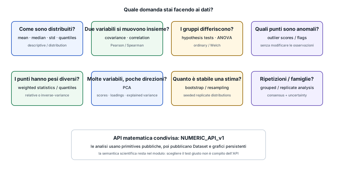
La statistica cerca di descrivere variabilità e incertezza e di distinguere pattern plausibili da differenze che potrebbero essere spiegate dal rumore o dal campionamento. Non esiste un unico “test statistico”: la domanda scientifica e il modo in cui i dati sono stati raccolti determinano quale metodo ha senso.
2. Concetti minimi
| Media / mediana | Misure di posizione centrale; la mediana è più robusta agli estremi. |
|---|---|
| Varianza / deviazione standard | Misure della dispersione attorno al centro. |
| Quantili | Soglie che suddividono la distribuzione, per esempio mediana = 50° percentile. |
| Covariance / correlation | Misurano co-variazione; la correlazione non dimostra causalità. |
| Hypothesis test | Confronta i dati con una ipotesi nulla secondo un test dichiarato. |
| ANOVA | Confronta la variabilità fra gruppi con quella all'interno dei gruppi. |
| PCA | Rappresenta variabili correlate con nuove direzioni che catturano molta varianza. |
| Bootstrap/resampling | Costruisce distribuzioni empiriche di una stima ripetendo campionamenti controllati. |
3. Moduli presenti nella dev-031
| ID | Nome | Versione | Tipo | Scopo |
|---|---|---|---|---|
analysis.statistics.descriptive | Descriptive Statistics | 1.1.0 | analysis | Statistiche descrittive + histogram/box-whisker Plot Dataset. |
analysis.statistics.grouped | Grouped Statistics | 1.0.0 | analysis | Statistiche per gruppi categoriali o numerici. |
analysis.statistics.correlation | Covariance and Correlation | 1.0.1 | analysis | Covariance/correlation con missing-data policy. |
analysis.statistics.distribution | Empirical Distribution | 1.0.1 | analysis | Istogramma/ECDF e distribuzioni empiriche riproducibili. |
analysis.statistics.outliers | Outlier Flags | 1.0.1 | analysis | Score, limiti e flag mantenendo source-row identity. |
analysis.statistics.weighted | Weighted Statistics | 1.0.1 | analysis | Statistiche e quantili con pesi. |
analysis.statistics.tests | Hypothesis Tests | 1.0.1 | analysis | Test di ipotesi tramite NUMERIC_API. |
analysis.statistics.anova | One-way ANOVA | 1.0.1 | analysis | ANOVA one-way ordinaria o Welch. |
analysis.statistics.pca | Principal Component Analysis | 1.0.1 | analysis | Scores, loadings, explained variance e scaling. |
analysis.statistics.resampling | Resampling Inference | 1.0.1 | analysis | Distribuzioni di replicate seeded e summary. |
analysis.regression | Regression | 1.0.1 | cross-area | Regression numerica con coefficienti/covariance/metrics. |
curve.replicate_analysis | Replicate Curve Analysis | 8 | cross-area | Consensus e uncertainty su curve ripetute; non fitta un modello fisico. |
demo.numeric.statistics | Numerical Statistics Demo | 1.0.1 | reference/demo | Descriptive + weighted statistics. |
demo.numeric.uncertainty | Numerical Uncertainty Demo | 1.0.1 | reference/demo | Uncertainty propagation + weighted estimation. |
4. API statistica effettiva
Le primitive statistiche vivono in NUMERIC_API_v1: descriptive statistics, rank, covariance, Pearson/Spearman correlation, MAD, histogram, ECDF, quantili, weighted quantiles/statistics, hypothesis tests, one-way ANOVA, SVD/PCA building blocks, seeded resampling e una famiglia foundation.statistics con confidence interval, robust methods, multiple testing, bootstrap/permutation, logistic regression, GLM, survival e k-means.
5. Missing/non-finite data
Molte primitive richiedono una policy esplicita error o omit. Le analisi di correlation possono distinguere pairwise e listwise policies. Questo è parte del significato scientifico: eliminare osservazioni non finite cambia il campione.
6. Pesi
I pesi non sono automaticamente “incertezze”. NUMERIC_API_v1 distingue semantiche relative e inverse-variance nelle operazioni di fitting/statistica che lo prevedono. Zero-weight observations vengono escluse, mentre il conteggio resta diagnosticabile.
7. ANOVA in parole semplici
Una one-way ANOVA chiede se le differenze fra le medie dei gruppi sono grandi rispetto alla variabilità interna ai gruppi. La variante Welch è pensata per gruppi con varianze non omogenee. Un risultato significativo non dice da solo quali gruppi differiscono o perché.
8. PCA in parole semplici
Se molte variabili misurano aspetti correlati dello stesso fenomeno, PCA costruisce nuove coordinate ortogonali (“componenti principali”) ordinate per varianza spiegata. Scores descrivono le osservazioni nel nuovo spazio; loadings descrivono quanto ogni variabile contribuisce alle componenti.
9. Replicate Curve Analysis
È una caratterizzazione statistica di curve ripetute, non un fit di modello fisico. Con replicate ID espliciti usa il percorso trace-based; senza ID non inventa un numero di repliche ma tratta le osservazioni come point cloud ripetute, stima consensus e componenti di dispersione.
10. Collegamenti
Riferimento tecnico completo
Questa parte raccoglie integralmente la documentazione tecnica pertinente distribuita con GX-TXT per gli argomenti e i moduli trattati in questa pagina.
Descriptive Statistics — User and Technical Manual
Descriptive Statistics — User and Technical Manual
Purpose
analysis.statistics.descriptive computes ordinary
descriptive statistics for one or more numeric variables from one
Canonical Dataset. It is intentionally focused: grouped statistics,
correlation, distributions, outlier detection and weighted statistics
belong to separate modules.
Input
Choose one Dataset through the normal Analysis Source control. Add one or more rows to Variables and choose the numeric variables to summarize. GX-TXT persists variable choices with Dataset-qualified stable variable identities and resolves the current names at runtime.
An optional x_range Dataset Selection may restrict the
rows used by every selected variable. The module never reads private
Dataset files and never mutates the source Dataset.
Statistics
For each variable the module reports:
- selected observation count;
- finite/valid observation count;
- excluded NaN/Inf count;
- minimum, maximum and range;
- mean and median;
- sample and population variance;
- sample and population standard deviation;
- standard error of the mean, defined as sample standard deviation divided by the square root of the valid count;
- Q1, Q3 and IQR;
- RMS;
- additional configured percentiles.
NUMERIC_API_v1 supplies minimum/maximum/range, mean,
median, quartiles, IQR, population/sample variance and standard
deviation, RMS and quantiles. Quartiles/quantiles therefore use the
API’s documented Hyndman-Fan type 7 definition. The module derives only
the standard error from the API’s sample standard deviation and valid
count.
NaN / Inf policy
Omit explicitly excludes NaN, +Inf and
-Inf from numerical statistics and reports the number
excluded. Error stops the analysis if any selected
observation for a variable is non-finite. No non-finite value is
silently mixed into valid data.
Rows excluded because they lie outside an optional Dataset Selection are not counted as missing/non-finite observations; they are outside the analyzed subset.
Undefined valid states
With exactly one valid observation, sample variance, sample standard
deviation and standard error are mathematically undefined. The output
Dataset stores NaN for those values and sets
defined=false. The report writes undefined.
This is distinct from execution failure.
A selected variable with zero observations or zero finite observations is an explicit error.
Additional percentiles
The Additional percentiles field accepts values from 0 through 100 separated by commas or semicolons, for example:
1;5;10;90;95;99Q1, median and Q3 are already standard outputs, so configured 25, 50 and 75 percentiles are not duplicated.
Output Dataset
The module publishes a compact long-form table.generic
Dataset. Each row is one statistic for one source variable.
Columns:
| Column | Meaning |
|---|---|
variable_id |
stable source Variable ID |
variable_name |
current source variable name |
statistic |
statistic identifier |
value |
numerical result |
defined |
whether the result is mathematically defined |
unit |
numerical result base unit |
unit_power |
0 for counts, 1 for source-unit results,
2 for variance |
observation_count |
selected observations before non-finite filtering |
valid_count |
finite observations used |
excluded_count |
selected NaN/Inf observations excluded |
The value column intentionally has no Dataset-level unit
because a long-form result contains dimensionless counts, source-unit
quantities and squared-unit variances in the same column.
unit + unit_power preserves the dimensional interpretation
without inventing private unit conversion rules. For Dataset variables
declared as value_kind=elapsed_time, Table Stream exposes
the public canonical numeric representation in seconds; the summary
therefore reports unit=s for computed values instead of
relabelling canonical seconds with the source display unit.
Report
descriptive_statistics_report.txt contains the actual
results, source Dataset, selected variables, Selection ID, non-finite
policy, counts, warnings, producer version and publication
information.
descriptive_statistics_summary.ini contains a compact
machine-oriented run summary in addition to the published Dataset.
Automatic graphs
Version 1.1.0 uses public PLOT_DATASET_API_v2
distribution series through Plot Dataset Octave Bridge
v1 (gxtxt_plot_dataset_v2), available from GX-TXT
0.9.7.86. The production module does not source the GX-TXT desktop host
or write private plot state. When Create automatic distribution
plots is enabled, the module publishes a small derived sample
Dataset containing exactly the selected observations and then creates
persistent plot.dataset variants for:
- histogram;
- box/whisker summary with optional outlier display.
The plot sample Dataset is a normal published GX-TXT Dataset with
provenance. It is not a private cache and the source Dataset remains
unchanged. NaN, +Inf and -Inf are
preserved in this intermediate Dataset; plot.dataset
applies its documented finite-sample distribution policy.
Variables are grouped only when their units are compatible according
to the public Unit Registry. For example, V and
mV may share a plot because plot.dataset can
use the common unit service; A is placed in a separate
plot. No local unit-conversion formula is implemented by this
module.
Each automatic graph is created as a normal persistent plot
variant, so the user can open, edit, rerender and preserve it
through the standard GX-TXT plot workflow. The generated PNG copies are
listed in automatic_graphs.ini.
Configuration:
- Histogram bins:
autoor an integer from 2 through 512; - Histogram normalization:
count,probabilityordensity; - Box/whisker IQR multiplier: positive number,
default
1.5; - Show box/whisker outliers: boolean.
These plots are descriptive overviews. Distribution-specific
frequency tables, empirical CDFs and explicit binning workflows remain
the responsibility of analysis.statistics.distribution.
Student teaching Session
The package includes
session_generators/gxtxt_descriptive_statistics_student_lab_1.0.0.zip,
a Session Generator API v1 package intended for the standard
GX-TXT Numerical Examples library. It creates a
ready-to-run Session containing:
VandmVvariables to demonstrate compatible units;- an
Avariable to demonstrate automatic separation of incompatible quantities; - constant, signed, single-value and two-value variables;
- explicit
NaNobservations; - a persisted
x_rangeDataset Selection; - stable Variable IDs and preconfigured Repeatable Config rows;
- reference values in
metadata/ground_truth.txt; - a root-level
STUDENT_GUIDE.txtwith the first run and follow-up exercises.
The production module does not depend on this generator. It is only deterministic teaching/test material.
Provenance
The published Dataset records the producer module/version, source Dataset, source Variable IDs and normal Publication provenance. Optional Selection identity and analysis configuration are also present in the report/run summary.
Errors
The module fails explicitly for missing Dataset, no selected
variable, duplicate variable selection, unresolved/missing stable
Variable ID, text/non-numeric variables, invalid percentile values,
invalid output Dataset ID, incompatible Selection source, unsupported
Selection type, empty selection result, zero finite observations, and
non-finite data when policy is error.
Public GX-TXT APIs used
- Standard Module API v1
- Analysis Source Map API v1
- Analysis Source Access Runtime v2
- Dataset Variable Schema API v3
- Dataset Selection API v1
- Repeatable Config API v1
- Table Stream API v3
- Dataset Publication API v2 and Octave binding
NUMERIC_API_v1frommath.numeric- Unit Registry API v1
- Plot Module API v1
PLOT_DATASET_API_v2- Plot Dataset Octave Bridge v1
(
gxtxt_plot_dataset_v2) - Progress API v1
- Plugin Install API v1
- Session Generator Library API v1
Limitations
This module is not grouped statistics, distribution analysis, correlation, outlier detection, weighted statistics, regression or fitting. It does not perform local unit conversion and does not combine variables into a shared statistic. Ordinary numeric variables are summarized in their declared source unit; elapsed-time values follow the CORE canonical-seconds contract. Because variables are summarized independently, selecting variables with incompatible units is valid and never causes them to be combined or compared.
Grouped Statistics — Manual
Grouped Statistics — Manual
Scientific purpose
analysis.statistics.grouped calculates descriptive
statistics separately for categories or exact numeric values of one
grouping variable. Typical uses include measurements by site, treatment,
instrument, sample class, season, or replicate group.
The module is deliberately focused. It is not an SQL aggregation engine, ANOVA module, hypothesis-test module, regression module, or data-cleaning tool.
Inputs
The module consumes one Canonical Dataset through the public Analysis Source infrastructure.
Required configuration:
- one or more numeric Value variables;
- exactly one Grouping variable.
Optional configuration:
- one
x_rangeDataset Selection from the same source Dataset.
All variable bindings are persisted by the framework as stable
dataset_id + variable_id identities. The module does not
read Dataset Registry internals or construct Dataset file paths.
Grouping variable
The grouping variable may be a Schema v3 string variable
or a numeric variable.
String groups are matched exactly and their UTF-8 labels are preserved. An empty/whitespace-only string is a missing group value.
Numeric groups are formed from exact values exposed by the public
Table Stream numeric view. NaN, +Inf, and
-Inf are invalid group values.
Group order is deterministic: groups are numbered in order of first
appearance in the selected data. The published group_index
is therefore a stable coordinate for that analysis run, while
group_label preserves the scientific category.
This first version supports one grouping key only.
Selection
When an x_range Dataset Selection is configured,
grouping and statistics are computed only from rows inside that
Selection. The source Dataset remains unchanged.
Missing / invalid group policy
missing_group_policy is explicit:
omit: rows with a missing/invalid grouping value are excluded from every group and counted in the report;error: execution stops explicitly when such a row is encountered.
Rows omitted because the grouping value is invalid are distinct from rows excluded because a selected numeric value is non-finite.
NaN / Inf value policy
nonfinite_policy is explicit for numeric value
variables:
omit:NaN,+Inf, and-Infare excluded independently for each group × variable result;error: execution stops if a selected value contains a non-finite observation in a row that otherwise belongs to a valid group.
The output records the group observation count, finite
count, and excluded non-finite count for every group ×
variable row.
Statistics
For every group × selected value variable the module reports, where defined:
- finite count;
- minimum;
- maximum;
- mean;
- median;
- sample standard deviation;
- standard error of the mean;
- Q1;
- Q3;
- IQR.
The numerical definitions come from public
NUMERIC_API_v1. Quartiles therefore use the API definition
rather than a private implementation.
Location/range statistics are defined with at least one finite
observation. Sample standard deviation and standard error require at
least two finite observations. Undefined mathematical results are
represented explicitly through location_defined and
sample_spread_defined; they are not execution failures.
Units
Each value variable retains its declared unit in the normalized
result through the row-level unit column. Numeric statistic
columns themselves have no single Dataset-wide unit because one result
Dataset may contain variables with different dimensions.
The module never performs private unit conversion. Automatic plot
grouping uses the public Unit Registry to determine whether selected
variables may share an axis. Compatible units such as V and
mV may share one plot; incompatible quantities are
separated.
For canonical elapsed-time values exposed from
value_format=hms, the public numeric representation is
seconds and the module follows that CORE contract.
Published grouped-result Dataset
The configured output Dataset contains one row per:
group × selected value variableImportant columns include:
group_index;group_key;group_label;group_numeric_valueandgroup_numeric_defined;group_variable_id,group_variable_name,group_unit;variable_id,variable_name,unit;observation_count;count;excluded_count;location_defined;sample_spread_defined;minimum,maximum,mean,median;standard_deviation,standard_error;q1,q3,iqr.
The Dataset is machine-readable and may be consumed by other GX-TXT modules.
Plot-support Dataset
When automatic graphs are enabled, the module publishes
<output_dataset_id>.plot, one row per group,
containing:
- numeric
group_index; - original
group_label; - group observation count;
- per-value-variable mean and SEM;
- per-value-variable median and asymmetric IQR deltas;
- per-value-variable finite count.
This Dataset exists because normal plot.dataset Graph
Series bind variables, not filtered rows inside a normalized long-form
summary. It is a normal derived Dataset published through Dataset
Publication API v2, not a private plotting sidecar.
Automatic graphs and variants
Automatic graphs use the public PLOT_DATASET_API_v2
through the standard_octave public bridge. No private
Octave plotting code is used.
For every compatible unit family the module creates two persistent variants:
- Grouped means ± SEM using error-bar series.
- Grouped medians + IQR using asymmetric error bars from median to Q1/Q3.
It also creates one Group observation count bar variant.
plot.dataset currently uses numeric X for these
Cartesian/bar representations, so the X coordinate is
group_index. The original category labels remain in the
plot-support Dataset, report, and automatic_graphs.ini. For
up to 10 groups the PlotSpec also adds public reference-line annotations
carrying the group labels. This is presentation only; group identity
remains in the published Dataset.
All automatic plots are persistent variants. They can be reopened and rerendered through normal GX-TXT plot facilities.
Report
grouped_statistics_report.txt records:
- producer/version;
- input and output Dataset IDs;
- grouping variable identity;
- selected value variables;
- Selection;
- non-finite and missing-group policies;
- selected and excluded row counts;
- group-index mapping;
- actual computed statistics;
- undefined-result warnings;
- automatic graph information.
Provenance and source immutability
Published Datasets identify the producer, producer version, source Dataset, source variables, Selection, and analysis policies through normal GX-TXT publication/provenance mechanisms.
The source Dataset is read-only. The module never deletes, replaces, filters, or mutates source values.
Error behavior
Execution fails explicitly for invalid scientific configuration, including:
- no Dataset;
- no value variable;
- more or fewer than one grouping variable;
- non-numeric value variable;
- Selection from another Dataset;
- unsupported Selection type;
- invalid policy;
- invalid/missing groups when policy is
error; - non-finite values when policy is
error; - no valid groups after Selection/policy;
- output Dataset ID conflicts.
Mathematically undefined statistics for a valid group are reported as undefined and are not confused with execution failure.
Performance and cancellation
The module is serial and low-overhead by design. Table Stream API v3 performs bounded source reads. Exact medians/quartiles require retaining the selected values per group, so memory use grows with the selected observations. No private worker pool is created.
Public GX-TXT APIs used
- Standard Module API v1
- Analysis Source Map / Access Runtime
- Dataset Variable Schema v3
- Dataset Selection API v1
- Repeatable Config API v1
- Table Stream API v3
- Dataset Publication API v2 and Octave binding
NUMERIC_API_v1- Unit Registry API v1
- Plot Dataset API v2 and Octave bridge v1
- Progress API v1
- Plugin Install API v1
- Session Generator Library API v1 for the teaching package
Limitations
- One grouping variable/key per analysis run.
- Numeric grouping is exact-value grouping; no automatic binning is performed.
- Grouped hypothesis tests and ANOVA are outside this module.
- Automatic categorical plots use numeric
group_indexbecause currentplot.datasetCartesian/bar X bindings are numeric. Original labels are preserved and explicitly mapped; no private categorical-axis implementation is introduced.
Covariance and Correlation
Covariance and Correlation
Select at least two numeric variables from one canonical Dataset.
Optional Dataset Selection limits the rows before missing-data handling.
Choose pairwise to omit nonfinite values independently for
each pair, or listwise to require every selected variable
finite on a shared row set. Set NaN / Inf policy to error
to reject nonfinite selected observations instead.
The result Dataset contains one row for every ordered variable pair, with sample covariance, Pearson correlation, Spearman correlation, the pair’s valid/input/excluded counts, and a covariance-unit string. Correlations are dimensionless. A constant variable yields an undefined correlation (NaN) with its status recorded; fewer than two valid paired observations yield undefined covariance/correlations. Source rows and source Dataset remain unchanged.
When enabled, the module creates a persistent Plot Dataset heatmap of Pearson correlation. Analysis configuration, source Dataset and stable variable IDs, Selection ID, missing-data policy and module version are recorded in result provenance. The full selected matrix is retained in memory for this analysis; Table Stream chunking bounds I/O, not the matrix size.
Empirical Distribution
Empirical Distribution
Select a numeric Dataset variable, optionally restrict rows with a Dataset Selection, and choose a reproducible bin rule. Count uses a fixed number of equal-width bins over the selected finite data range; width uses a specified width; edges uses a strictly increasing list of explicit edges. The last edge is included in the last bin. Values outside explicit edges remain out of range and are counted in the report. Relative and cumulative frequencies use all valid observations as denominator.
The module publishes three table.generic Datasets:
<prefix>.bins (frequency table with left/right edges,
centers, counts and frequencies), <prefix>.ecdf
(distinct support values, counts and cumulative probability), and
<prefix>.quantiles (requested probability and type-7
quantile). Public NUMERIC_API_v1 computes all three. The
source Dataset is read through public Analysis Source and Table Stream
interfaces and remains unchanged. Provenance includes the source stable
Dataset/variable IDs, bin rule, Selection, and nonfinite policy.
The optional histogram and ECDF graphs are persistent Plot Dataset variants. Results and settings are stored in the Session. Vector results require memory proportional to the number of selected observations and distinct values.
Outlier Flags
Outlier Flags
Select a numeric Dataset variable, an optional Dataset Selection, and an explicit positive multiplier. The IQR rule uses type-7 Q1 and Q3, with fences Q1 − multiplier × IQR and Q3 + multiplier × IQR. Its signed score is (value − median) / IQR. The MAD rule uses the median and normal-consistency scaled MAD, with symmetric limits median ± multiplier × scaled MAD. Its signed score is (value − median) / scaled MAD. A zero scale produces score 0 at the center and signed infinity for a differing value; comparison with the finite limits still defines the flag.
The published table.generic Dataset contains the
original one-based source_row, selected value, method,
signed score, lower/upper limits, and a 0/1 is_outlier
flag. All selected rows remain present. Under omit,
nonfinite input rows have NaN score and flag 0; they are counted
separately and are never silently removed from the published table.
Under error, any nonfinite input stops analysis.
NUMERIC_API_v1 supplies quantiles, MAD and vector
comparisons. Publication records stable source Dataset and variable IDs,
Selection, rule, threshold and nonfinite policy. The source Dataset
remains unchanged. The full selected vector is retained in memory.
Weighted Statistics
Weighted Statistics
Choose a numeric measurement and a second, explicitly identified
variable. Statistical weight treats the second variable
as nonnegative, dimensionless weights. Zero-weight rows remain in the
valid-row count but do not influence estimates. No measurement
uncertainty is inferred from such weights. The inverse variance
uncertainty model treats the second variable as a strictly
positive standard measurement uncertainty with units compatible with the
measurement. The module converts uncertainties into the measurement unit
and sets each weight to 1 / uncertainty².
The public NUMERIC_API_v1 weighted statistics and
weighted quantiles operations compute counts, sum of weights, weighted
mean, population and unbiased weighted variance/standard deviation,
weighted median, IQR, effective sample size, and weighted empirical-CDF
inverse quantiles. The summary Dataset separates
measurement_uncertainty_of_mean (known independent
measurement uncertainties, sqrt(1 / sum(weights)) in the
inverse-variance model) from
sampling_standard_error_of_mean (optional
sqrt(unbiased_weighted_variance / effective_n) under the
sampling model). The latter is a sampling estimate of replicate
variability; it is not a measurement-uncertainty conversion. Unsupported
estimates are NaN with a status field explaining why.
The result is two table.generic Datasets,
<prefix>.summary and
<prefix>.quantiles. Provenance records the stable
source Dataset and variable IDs, Selection, weight model, mean-SE model,
and nonfinite policy. Source rows are read through Analysis Source and
Table Stream APIs and never modified. The selected vectors are retained
in memory.
Hypothesis Tests
Hypothesis Tests
The method is explicit: one-sample t, independent pooled-variance t,
Welch t, paired t, Mann-Whitney/Wilcoxon rank-sum, or Wilcoxon
signed-rank. The second variable is required except for one-sample t.
Independent tests use the two columns as separate samples; paired tests
align the two values in each selected source row. Missing values are
handled by the selected error or omit policy
inside public NUMERIC_API_v1. The alternative is two-sided,
greater or less, with the first sample or first-minus-second difference
defining direction.
The null mean or mean difference applies to t-tests only. Rank tests require zero null shift. Two-variable tests require compatible units; the second variable is converted to the first variable’s unit through the Unit Registry. T-tests publish mean or mean-difference confidence intervals and Cohen’s d where defined. Welch’s test does not invent a standardized effect. Rank tests publish rank-biserial effect size; their location-shift confidence interval is explicitly undefined. Rank p-values are exact conditional permutation/sign values for at most 20 relevant observations; larger samples use a tie-corrected normal approximation with continuity correction.
The result table.generic Dataset publishes method,
statistic, degrees of freedom, input and valid counts, p-value,
alternative, confidence level and bounds, effect size/name, null value,
estimate, nonfinite policy and approximation method. The report and
summary carry stable source Dataset/variable IDs and configuration
provenance. The source Dataset remains unchanged.
One-way ANOVA
One-way ANOVA
Choose a numeric measurement and a text or numeric group variable
from one Dataset, optionally restricted by a Dataset Selection. Ordinary
one-way ANOVA assumes a common within-group variance. Welch one-way
ANOVA uses group-specific variances and requires at least two
observations and positive variance in every group. The method is never
chosen automatically. Missing labels or nonfinite measurements follow
the explicit error or omit policy.
The public NUMERIC_API_v1 operation computes group
counts, means and variances, between/within/total sums of squares,
degrees of freedom, F and p-value. Ordinary ANOVA also reports
eta-squared and omega-squared. These effect sizes are marked undefined
for Welch’s heteroscedastic test. Post-hoc comparisons are not part of
this module.
Two table.generic Datasets are published:
<prefix>.groups contains stable first-seen group
indices, labels, counts, means, variances and standard deviations;
<prefix>.test contains the method, observation
counts, sums of squares, degrees of freedom, F, p-value and effect
sizes/status. An optional group-mean graph is a persistent public Plot
Dataset variant. Provenance records stable source Dataset and variable
IDs, Selection, method and nonfinite policy. The source Dataset remains
unchanged.
Regression
Regression
Select numeric X and measured Y variables from one Dataset, optionally restrict rows by a Dataset Selection, and choose linear or polynomial regression. Linear mode includes an intercept. Polynomial mode uses the requested positive degree and the public numerical API’s centered/scaled design for stability. Rank-deficient fits fail by default; an explicit minimum-norm policy is available and recorded.
Weight semantics are explicit. None gives ordinary
least squares. Statistical weight uses a separate
nonnegative dimensionless variable; zero-weight rows are excluded from
fitting. Inverse variance uncertainty uses a strictly
positive measurement standard uncertainty compatible with Y, converts it
to the Y unit, and computes 1 / uncertainty² weights. The
model and the public NUMERIC_API_v1 fit record the weight
semantics. Missing or nonfinite rows follow the selected policy; every
published fit row preserves the original one-based source-row
identity.
The module publishes <prefix>.fit (X, measured Y,
fitted Y, residuals and absolute residuals),
<prefix>.curve (sorted observed X and model
predictions for plotting), <prefix>.coefficients
(index, power, estimate, standard error and coefficient-unit text),
<prefix>.covariance (coefficient covariance matrix as
ordered pairs), and <prefix>.metrics (R², adjusted
R², RMSE, residual error metrics, rank, condition number, degrees of
freedom, SSE and weight semantics). Fit and residual plots are
persistent public Plot Dataset variants. Reports and provenance record
stable source Dataset/variable IDs, Selection and all scientific
choices. No nonlinear model fitting is added here.
Principal Component Analysis
Principal Component Analysis
Choose at least two numeric variables from one Dataset and optionally restrict rows by a Dataset Selection. The missing-data rule is explicit: fail on any nonfinite value or remove complete rows listwise. Removed rows are counted and never imputed. The score Dataset carries the original one-based source-row identity for every retained observation.
Centering subtracts each variable mean when enabled.
standardize divides by its sample standard deviation and
requires positive spread. none keeps source units and
requires all variables to have compatible linear units; values are
converted to the first variable’s unit before decomposition.
Standardization permits mixed linear units. Uncentered PCA uses the
uncentered second-moment SVD; explained variances still use
singular-value squares divided by n−1, and the report
records that choice.
The public NUMERIC_API_v1 matrix SVD provides singular
vectors and values. Components are chosen either by an explicit count or
by the smallest number reaching the requested cumulative
explained-variance fraction. Singular-vector signs are oriented
deterministically so each loading’s largest-magnitude element is
positive.
Published table.generic Datasets are
<prefix>.scores, .loadings,
.components, and .scaling. They contain
scores, loadings, eigen/explained variance and ratios, singular values,
variable means/scales and stable source variable IDs. Scree, PC1/PC2
score and loading graphs are persistent public Plot Dataset variants
when enabled. Provenance records Selection, preprocessing, component
policy and missing-data rule. The selected matrix and SVD are retained
in memory.
Resampling Inference
Resampling Inference
Choose a stable numeric Dataset variable and an optional Selection. Bootstrap resamples the finite first sample with replacement and reports a percentile confidence interval for its mean, median or sample standard deviation. At least two finite values are required. This is a basic percentile interval; it does not claim bias correction or guaranteed coverage for dependent observations.
Independent permutation compares the difference in group means using
two variables as separate samples. Nonfinite values are removed
independently; each variable may have a different number of
observations. Paired permutation uses rows where both variables are
finite, converts the second variable to the first unit, and randomly
flips the sign of each paired difference. Permutation p-values use the
finite Monte Carlo correction
(extreme + 1)/(replicates + 1); the alternative is
explicit. The null distribution and observed difference have the first
variable’s unit. For independent samples, the grouping labels are the
two chosen variables.
The explicit positive seed uses the public NUMERIC_API Park–Miller
generator. Batches continue from its returned next_seed, so
the result does not depend on global random state. Iterations are
bounded to ten million generated indices and at most 100,000 replicates.
The module emits determinate progress after each batch. The framework’s
standard run cancellation terminates the module process; no partial
Dataset is published until all requested iterations finish. Parallel
execution is not used for these bounded sequential batches.
The .distribution Dataset contains every replicate and
the .summary Dataset contains counts, estimate, interval or
p-value, seed, method and configuration. Both carry source Dataset and
stable variable IDs, Selection ID, unit and complete run provenance. The
source Dataset is immutable. Invalid units, missing bindings, nonfinite
policy violations and unsupported settings fail explicitly.
Numerical Statistics Demo — Manual
Numerical Statistics Demo — Manual
Plugin ID: demo.numeric.statistics
Plugin version: 1.0.0
Reference framework: GX-TXT 0.9.7.82
License: GNU GPL v3 or later
1. Purpose
This plugin is a compact demonstration/reference consumer of GX-TXT’s
public numerical architecture. It demonstrates statistics on a Canonical
Dataset through math.numeric / NUMERIC_API_v1,
publishes reusable derived Datasets, writes a human-readable report and
renders an automatic graph.
It is not the future production family of descriptive/grouped/correlation statistics modules.
2. Public GX-TXT APIs used
The implementation uses only public framework paths relevant to the task:
- Standard Module API v1;
- Analysis Source Map API v1;
- Dataset Variable Schema API v3;
- Dataset Metadata API v1 when metadata are present;
- Dataset Selection API v1 for optional X-range filtering;
- Table Stream API v3 for bounded source inspection and graph-series preparation;
NUMERIC_API_v1frommath.numericfor all statistical calculations;- Dataset Publication API v2 for both derived Datasets;
- Graph Provider / shared graphics helpers for automatic PNG output;
- Plugin Install API v1;
- Session Generator Library API v1.
No CORE code is modified by this plugin.
3. Statistical capabilities found in GX-TXT 0.9.7.82
The inspected math.numeric 1.1.0 public API provides
descriptive statistics, quantiles and weighted statistics, including
Dataset-aware descriptive and weighted operations.
Descriptive statistics return:
- count of values used;
- minimum, maximum and range;
- sum and arithmetic mean;
- median, Q25, Q75 and IQR;
- population variance and standard deviation;
- sample variance and standard deviation;
- RMS.
Quantiles use Hyndman-Fan type 7 linear interpolation.
Weighted statistics return:
- finite-pair count before zero-weight removal;
- positive-weight count;
- sum of weights and effective sample size;
- minimum, maximum and range on positive-weight observations;
- weighted sum and mean;
- weighted empirical-CDF median, quartiles and IQR;
- population weighted variance/std;
- reliability-weight unbiased variance/std where defined;
- weighted RMS.
Standalone statistical covariance/correlation operations are not
exposed by the current NUMERIC_API_v1. Covariance objects
present in fitting and uncertainty-propagation APIs are different
capabilities. This demo therefore has no covariance/correlation
mode.
4. Session Generator
The package includes the portable Session Generator:
Library:      GX-TXT Numerical Examples
Category:     Mathematics
Generator:    Statistics
generator_id: statistics
version:      1.0.0
Import
session_generators/gxtxt_numerical_examples_statistics_1.0.0.zip
with the Library Manager. The generated ordinary Session contains:
raw/statistics_demo.csv
metadata/ground_truth.txt
The plugin never reads ground_truth.txt during analysis.
That file exists only for human inspection and independent tests.
5. Source Dataset import
Import raw/statistics_demo.csv through the normal
Acquisition / generic CSV workflow as a table.generic
Canonical Dataset. A documented example Dataset ID is:
statistics.sourceSuggested variable semantics/units:
| CSV column | Unit | Suggested role |
|---|---|---|
sample |
1 |
independent |
value_V |
V |
measured |
weight |
1 |
weight |
Do not rely on the example’s imported variable IDs. The module resolves stable IDs from Analysis Source / Variable Schema runtime data.
6. Configuration
The compact module configuration contains:
- Value variable — required;
- Weight variable — optional except in Weighted mode;
- Data selection — optional X-range Dataset Selection;
- Statistics mode —
descriptiveorweighted; - NaN / Inf policy —
omitorerror; - Summary Dataset ID.
Descriptive is the default mode.
7. Dataset Selection
If an X-range Dataset Selection is chosen, it is passed to the Dataset-aware numerical operation through the public Selection structure. The same public selection mask is used only to prepare matching counts and graph-series rows; the plugin does not implement a private filter language.
Input count in the report means rows remaining after the
Dataset Selection and before the selected non-finite policy.
8. NaN / Inf policy
The public math.numeric default is
nonfinite=error. This demo exposes the policy explicitly
and defaults its example workflow to omit because the
deterministic Statistics dataset contains three missing-value markers
that the public CSV provider exposes numerically as
NaN.
With omit:
- descriptive mode removes non-finite values;
- weighted mode removes pairs where either value or weight is non-finite;
- invalid data are never converted to zero.
The report states input, valid/used and excluded non-finite counts. In weighted mode it separately reports finite pairs, positive-weight observations and zero-weight observations.
With error, the public numerical operation rejects
non-finite input and the plugin does not publish partial output.
9. Weight semantics
The Weight binding is an explicit statistical weight. It is not a measurement uncertainty.
A Dataset uncertainty column, if present in some other source, is not automatically reinterpreted as a weight. If a scientific workflow requires inverse-variance weights derived from uncertainty, that transformation must be explicit in the appropriate analysis workflow; this demo does not invent it.
Zero weights are discarded by the public weighted-statistics operation. Negative weights are errors. At least one positive weight is required.
Weighted quantiles use the public
weighted empirical CDF inverse definition.
10. Variance and standard-deviation conventions
Descriptive mode reports both conventions returned by
NUMERIC_API_v1:
- population variance/std: divisor
n; - sample variance/std: divisor
n-1, undefined (NaN) for a single observation.
Weighted mode reports:
- population weighted variance/std;
- reliability-weight unbiased variance/std where mathematically defined.
The plugin does not choose an alternative convention.
11. Units
Minimum, maximum, range, sum, mean, median, standard deviation, RMS and quantiles retain the Value variable unit.
Variance is published/reported with the squared-unit expression, for
example V^2. GX-TXT’s Unit Registry parser supports simple
powers; no false unchanged V metadata is assigned to
variance.
Counts and effective sample size are dimensionless. Weighted sum
carries value*weight units when the Weight variable itself
is not dimensionless. Correlation is not produced because no public
correlation operation is exposed in this framework version.
12. Derived Datasets
Summary Dataset
Default ID:
demo.numeric.statistics.resultSchema:
| Variable | Type | Meaning |
|---|---|---|
statistic |
string | Stable statistic name |
value |
float64 | Computed numeric value |
unit |
string | Per-statistic scientific unit |
definition |
string | Definition/convention note |
A long-form schema is used because different statistics have
different units. The numeric value column therefore does
not falsely claim one common unit; the per-row unit field
carries the correct unit.
Graph/reuse series Dataset
Default ID:
demo.numeric.statistics.result.seriesIt contains the observations actually included by the public
operation, a sequential included-observation index, constant mean and
median reference series, and explicit weights in weighted mode. It is
suitable for normal downstream Dataset consumers, including
plot.dataset.
13. Provenance
Publication records include:
- producer module and version;
- source Dataset ID;
- source Value variable ID;
- Weight variable ID in weighted mode;
- Selection ID when used;
- numerical mode;
- explicit non-finite policy;
- public numerical API identity.
The source Dataset is never modified.
14. Report
statistics_report.txt contains:
- plugin ID/version;
- source Dataset and stable variable IDs;
- selected variables and units;
- Selection identity or Full Dataset;
- exact public numerical operation;
- input/valid/excluded counts;
- weighted counts/configuration when applicable;
- variance/std convention;
- quantile convention;
- computed statistics and units;
- Dataset Metadata availability;
- published Dataset IDs;
- graph output;
- the documented absence of standalone covariance/correlation operations.
statistics_metrics.ini provides a compact
machine-readable run summary.
15. Automatic graph
01_statistics_values.png plots observations actually
used by the selected public operation and overlays its mean and median.
Weighted mode labels the reference lines as weighted mean/median.
The graph is module-owned but uses GX-TXT shared graphics/Graph
Provider infrastructure. Rerender uses only
render_cache.mat; it does not recalculate statistics.
16. Save/reopen
Module settings use the normal Standard Module manifest path. The test suite verifies persistence of mode, non-finite policy, output Dataset ID, binding configuration and Selection ID through manifest write/reload.
Published Datasets are ordinary registered Canonical Datasets and remain addressable after Session reopen according to normal GX-TXT Dataset persistence.
17. Tests
The package contains:
tests/test_static.py
tests/test_framework_integration.tcl
Coverage includes deterministic generator data, normal/constant/signed/single-value/non-finite numerical semantics, explicit weighted behavior, package installation, generator import, Canonical Dataset import, stable variable resolution, API capability discovery, Selection persistence and real Octave execution when available.
Runtime-dependent checks are reported as SKIP when GNU
Octave is absent; no PASS is fabricated.
See TEST_RESULTS.md for the execution performed for this
release.
18. Known limitations
- No standalone covariance/correlation mode because GX-TXT 0.9.7.82 does not expose those public statistical operations.
- No regression; that belongs to
demo.numeric.regression. - No histogram is generated because this demo does not require a new
graph type or any patch to
plot.dataset. - Only normal X-range Dataset Selection is supported by the descriptor for this reference demo.
Numerical Uncertainty Demo — User Manual
Numerical Uncertainty Demo — User Manual
Purpose
This reference plugin demonstrates the uncertainty-aware capabilities
that GX-TXT 0.9.7.82 actually exposes through math.numeric
/ NUMERIC_API_v1. It is not a complete GUM
uncertainty-budget, calibration or metrology application.
Installation
Install demo.numeric.uncertainty_1.0.0.zip through the
normal GX-TXT Plugin Install interface/API. The package requires GX-TXT
0.9.7.82 or later and the bundled math.numeric service.
Demonstration Session
Import the bundled generator package into the existing GX-TXT Numerical Examples library, then use:
Generate Session... → GX-TXT Numerical Examples → Mathematics → Measurement Uncertainty
The generator creates
raw/measurement_uncertainty_demo.csv with:
measurement_id— dimensionless measurement number;value_V— measured voltage in V;sigma_V— measurement standard uncertainty in V;weight_V_m2— explicit reference inverse-variance weight inV^-2.
The generator computes the weight column explicitly as
1/sigma^2. That conversion exists only in the deterministic
demonstration source. The analysis plugin never performs it
automatically and never reads generator-private ground truth.
Import the CSV through normal Acquisition as a
table.generic Canonical Dataset.
Bindings
Bind:
- Measured value variable to the quantity being estimated;
- Uncertainty / weight variable to either a standard-uncertainty variable or an explicit-weight variable, according to Input interpretation.
Bindings are persisted through Dataset ID + stable variable ID, not CSV column number or display text.
Input interpretation
Standard uncertainty
The auxiliary variable is interpreted as measurement standard uncertainty of the measured value. For this first demo, its unit string must exactly match the measured-value unit string.
The public numerical path is:
statistics(values)→ arithmetic mean and descriptive reference statistics;propagate_uncertainty(J, sigma, input_kind=standard_uncertainty)→ standard uncertainty of the arithmetic mean, where the plugin supplies the Jacobian of the mean.
NUMERIC_API_v1 requires standard uncertainties to be
finite and non-negative. Zero is accepted; negative uncertainty is
rejected.
Explicit statistical weight
The auxiliary variable is interpreted only as an explicit statistical weight. It is never reinterpreted as standard uncertainty.
The public numerical path is:
statistics(values)→ ordinary mean of the finite paired observations;weighted_statistics(values, weights)→ weighted mean, weighted spread, sum of weights and effective sample size;- with
weight_semantics=inverse_variance,least_squares(ones, values, weights)→ coefficient standard error and reduced chi-squared using the public absolute inverse-variance covariance convention.
Public weighted statistics reject negative weights, discard zero weights, and require at least one positive weight.
weight_semantics=relative treats weights as relative
statistical importance. Relative weights alone do not define absolute
measurement uncertainty, so the plugin does not label a residual-scaled
fit error as measurement uncertainty in this mode.
NaN / Inf policy
error preserves the public rejection behavior.
omit removes affected value/auxiliary pairs before
uncertainty propagation because propagate_uncertainty
itself requires finite inputs. Invalid finite uncertainties/weights are
still validated by the public numerical operations and are never
repaired or replaced.
Dataset Selection
An optional normal GX-TXT X-range Dataset Selection can be applied before analysis. No private row-filtering UI or persistent range format is introduced.
Published Dataset
The default output Dataset ID is
demo.numeric.uncertainty.result. The Canonical Dataset uses
a long-form schema:
quantityvalueunitdefinition
Standard-uncertainty mode publishes counts, arithmetic mean, propagated standard uncertainty of the mean, and value spread. Explicit-weight mode publishes counts, sum of weights, effective sample size, ordinary/weighted means and weighted spread; inverse-variance mode additionally publishes the public least-squares estimate standard error and reduced chi-squared.
The Dataset preserves normal producer/source-variable provenance and never modifies the source Dataset.
The module also publishes
<output_dataset_id>.series, containing the selected
measurement values, auxiliary uncertainty or weight, and mean-reference
variables. Plot.dataset reads this canonical Dataset when drawing and
rerendering the graph; the render cache stores only its identity and
presentation metadata.
Report
uncertainty_report.txt records the source Dataset, bound
stable variables, interpretation, public operations, Selection, counts,
non-finite policy, results, units, weighting semantics and
warnings/limitations.
Graph
01_uncertainty_measurements.png is owned by the module’s
Graph Provider entry and rendered through the public Plot.dataset API.
Its persistent Plot Variant can be edited with the framework plot
controls and rerendered after reopening the Session.
- Standard-uncertainty mode shows measurement values with supplied standard uncertainty as Y error bars plus the arithmetic mean.
- Explicit-weight mode shows measurement values plus ordinary and weighted mean reference lines. Statistical weights are not drawn as uncertainty bars.
Save / reopen
Normal module configuration, Analysis Source bindings, Selection identity and published Dataset state follow standard GX-TXT Session persistence rules.
Known limitations
GX-TXT 0.9.7.82 does not expose a generic public
standard uncertainty → inverse-variance weight conversion
operation. This plugin therefore does not implement one privately.
Supply an explicit weight variable when weighted estimation is
desired.
This demo does not provide a full uncertainty budget, Type A/Type B workflow, coverage-factor calculation, covariance editor, Monte Carlo propagation, calibration database or regression workbench.