Indice
Versione verificata
| Framework | GX-TXT 0.9.8.10-dev-031 |
|---|---|
| Solver/primitives | NUMERIC_API_v1 |
1. Che cos'è un fit?
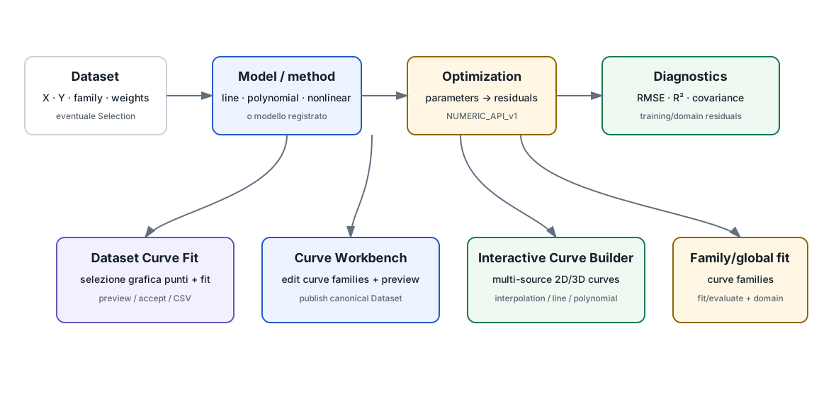
Fittare significa scegliere un modello con parametri e trovare i parametri che rendono le predizioni compatibili con i dati secondo una funzione obiettivo, normalmente legata ai residuals. Il fit non “dimostra” che il modello sia vero: misura quanto quel modello riesce a descrivere i dati nel dominio considerato.
2. Interpolazione, regression e nonlinear fitting
| Interpolazione | Costruisce una curva fra punti; non stima necessariamente un modello fisico. |
|---|---|
| Linear regression | Stima una relazione lineare fra X e Y. |
| Polynomial fit | Stima coefficienti di un polinomio del grado scelto. |
| Nonlinear fit | Ottimizza parametri di un modello non lineare; dipende da initial guesses e possibili minimi locali. |
| Family/global fit | Un unico modello parametrico viene adattato a più curve/famiglie con input semantici condivisi. |
3. Moduli e strumenti presenti
| ID | Nome | Versione | Tipo | Scopo |
|---|---|---|---|---|
analysis.regression | Regression | 1.0.1 | analysis | Linear/polynomial regression general-purpose su Dataset. |
demo.numeric.regression | Numerical Regression Demo | 1.0.1 | reference/demo | Reference OLS/WLS workflow. |
demo.numeric.nonlinear_fit | Nonlinear fit integration demo | 1.0.5 | reference/demo | Callback nonlinear fit e validation. |
curvefit.family_global | Curve Family Fitting | 6 | analysis | Fit/evaluate di modello parametrico su curve_family.table, domain classification e Plot Dataset. |
curve.replicate_analysis | Replicate Curve Analysis | 15.2 | pre-fit/statistical | Consensus/uncertainty di curve ripetute; prepara fit-ready data ma non fitta un modello fisico. |
viewer.dataset_curve_fit | Dataset Curve Fit | 0.1.0 | viewer | Filtri, selezione grafica punti, fit line/polynomial/exponential/power/Gaussian, residuals, CSV. |
viewer.curve_workbench | Curve Workbench | 1.0.4 | viewer | Editing di curve families, interpolation/line/polynomial preview, publication. |
viewer.interactive_curve_builder | Interactive Curve Builder | 1.0.0 | viewer | Curve 2D/3D da più Dataset, selection, interpolation/fit, transient preview e publication. |
4. API di base
NUMERIC_API_v1— least squares, linear regression, polynomial fit, nonlinear callbacks, residual metrics e optimization.PARAMETER_SET_API_v1— file di parametri congelati/riusabili.MODEL_DOMAIN_API_v1— dominio di training nello spazio degli input del modello.
5. API dei viewer/workbench
6. Dataset Curve Fit
È il viewer più diretto per “prendere una curva e provarci un fit”. Supporta filtri numerici/testuali, point selection Native 2D, fit su tutti o solo punti selezionati e modelli linear, polynomial (grado 1–12), exponential, power law e Gaussian. Preview mostra formula, coefficienti, RMSE/R² e residuals; Accept conserva fit separati dalla sorgente.
7. Curve Workbench
È prima di tutto un editor di curve families con source-row identity: sposta, aggiunge/elimina punti, undo/redo e preview nearest/linear/cubic/spline/PCHIP/line/polynomial. Publish crea un nuovo Dataset canonico con provenance degli edit.
8. Interactive Curve Builder
Combina source rows da più Dataset, selection/family member, curve 2D o parametriche 3D. Può interpolare oppure fare line/polynomial fit e mostrare preview transiente tramite Plot Dataset; Publish salva il risultato come Dataset.
9. Replicate Curve Analysis prima del fitting
curve.replicate_analysis 15.2 entra nel workflow quando la stessa curva o famiglia di curve è disponibile in più ripetizioni o più sorgenti. Il modulo costruisce consenso, dispersione e componenti d'incertezza e può produrre dati fit-ready prima di passare al modello fisico.
È quindi un passaggio di preparazione statistica, non un fitter: il suo output può alimentare curvefit.family_global o altri strumenti di fitting senza confondere la variabilità delle repliche con i parametri del modello.
10. Curve Family Fitting
Lavora su curve_family.table e modelli parametrizzati. In fit ottimizza parametri; in evaluate usa parametri congelati senza optimizer. Può classificare punti in/out del training domain usando un convex hull nello spazio degli input matematici.
11. Diagnostica
Guarda sempre residuals, RMSE/R² e il dominio di validità. Un solver che converge non garantisce un modello fisicamente sensato; un fit eccellente non rende automaticamente corretta una extrapolation.
Riferimento tecnico completo
Questa parte raccoglie integralmente la documentazione tecnica pertinente distribuita con GX-TXT per gli argomenti e i moduli trattati in questa pagina.
Curve Family Fitting — `curvefit.family_global`
Curve Family
Fitting — curvefit.family_global
GPL-3.0-or-later
This is a generic nonlinear curve-family fitting module. The 6BX7-GT is the first use case, not part of the module identity.
The module consumes a dataset with contract
curve_family.table. It declares three required input
roles:
x— independent X;family— family/sweep variable;y— measured dependent quantity.
For triode.koren_v1, model preferences are
X_V, Vg_V, Y_mA. These are
defaults, not hard-coded requirements. The Analysis tab allows each role
to be bound to any canonical dataset variable.
For the current VG_X.csv:
X_V,Vg_V,Y_mAall three bindings resolve automatically. If the user aliases
X_V to Va_V, the binding can be set to
Va_V and the canonical CSV is generated with that
header.
The runtime configuration written into the session records the resolved bindings, selected model, solver and model parameters, making a run reproducible.
Octave CLI entry point (v0.6.1)
curvefit_family_global.m is intentionally a minimal
command-line launcher. It adds its own plugin runtime plus the shared
core/octave/* directories to the Octave path and calls
curvefit_family_global_main(argv()). Helper functions are
subfunctions of the external function file rather than local functions
declared after executable script statements. This avoids the
direct-script startup failure arg_value undefined observed
with Octave 9.4.0.
A successful fit must create all descriptor-declared outputs:
fit_parameters.csv, fit_summary.txt,
fit_predictions.csv, render_cache.mat, and
01_curve_family_fit.png. The standard runner verifies this
contract before reporting success.
Standard legend editor
The plot curvefit.family.overlay declares
supports_legend=1 and legend_editor=standard.
legend_mode in the module plot configuration selects the
semantic content (family_only,
measured_and_fitted, or none). Placement and
visual formatting are handled separately by the common Plots →
Configure legend… editor and by Place legend by
click. These settings persist in Manifest Format 2 and apply
identically to initial rendering and rerendering.
Legend support
curvefit.family_global does not own a private
legend-positioning implementation. Its plot descriptor declares the
common legend capability and the renderer calls
gxtxt_plot_legend(). The Plots-tab editor can therefore
combine placement and layout independently, for example
below + row, below + wrapped (4 columns),
right + stacked, or manual + wrapped. Under
GNUplot the common renderer uses a dedicated legend axes so exported PNG
placement is deterministic.
Graph offerings (v0.7.2)
The module implements Graph Provider API v1 and currently offers:
curvefit.family.overlay— measured points and fitted family curves; enabled by default;curvefit.family.residuals— residuals (Y_fitted - Y_measured) grouped by family.
Enable/disable these plots in Analysis under the module plot
configuration. Graph selection is part of the experiment manifest and
does not change the fitted parameters. Rerender uses
render_cache.mat, so enabling the residual plot after a fit
does not repeat the numerical optimization.
Plot DPI is a global graphics setting, not a fitting
parameter. Legend font sizes can inherit the global
px/pt unit or override it per plot.
GX-TXT Curve Family Fitting — v0.7.8 plugin
GX-TXT Curve Family Fitting — v0.7.8 plugin
SPDX-License-Identifier: GPL-3.0-or-later
curvefit.family_global is a generic GX-TXT Pipeline
v0.7.8 analysis plugin for fitting and validating parameterized
mathematical models against curve_family.table
datasets.
Plugin version: 5
Module API: 1
Graph Provider API: 1
In version 5, fitting uses the runtime-advertised public
NUMERIC_API_v1 nonlinear solver with its explicit bounded
fallback; global, domain and group residual summaries use its
residual_metrics operation. All five graphs are persistent
public Plot.dataset variants; the module has no private fitting solver
or renderer. The v0.7.8 compatibility details below document the earlier
interface.
Operation modes
fit (default)
Preserves the established numerical fit workflow. The selected solver
optimizes the registered model parameters using the semantic model
bindings x, family, and y.
Old sessions without operation_mode are interpreted as
fit.
Fit mode also builds a 2D convex hull in mathematical-model input
space (x, family) and, when the hull is valid, writes the
optional sidecar fit_domain.csv.
evaluate
Uses frozen model parameters and never calls an optimizer. It computes predictions, residuals, metrics, training-domain classification, cache data and the normal graph-provider outputs.
Frozen parameters can come from:
parameter_source=manualwithfixed_parameter_valuesinmodel.param_namesorder;parameter_source=csvwithparameter_csv_path.
The CSV path is declared with the GX-TXT v0.7.8 generic
type=file field and therefore uses the framework Browse
control.
Shared Parameter-Set API
CSV parameter sets are read through the v0.7.8 shared helper:
gxtxt_read_parameter_set()The standard file remains compatible with:
parameter,value
mu,10.8
Kp,77.2
Parameter names, numeric values and optional model_id
metadata are validated by the framework helper. The plugin no longer
contains a private parameter-set parser.
Shared Model-Domain API
The training-domain sidecar uses the GX-TXT v0.7.8 Model-Domain format:
# model_id=triode.koren_v1
# domain_kind=convex_hull
x,family
...
x and family are stable mathematical-model
input roles, not dataset-specific column names. This is required so the
same fitted surface can be evaluated on datasets whose canonical column
names differ while the semantic model bindings remain the same.
The plugin uses the shared helpers:
gxtxt_read_model_domain()
gxtxt_validate_model_domain()
gxtxt_classify_model_domain()
The domain is always defined and classified in mathematical-model
input space. Measured y and
presentation_orientation never participate in the in/out
test.
When Evaluate uses a parameter CSV, the plugin automatically looks
for fit_domain.csv in the same directory. If no sidecar
exists, evaluation continues with domain_role=unknown and
the summary reports that the training domain is unavailable.
A legacy pre-v0.7.8 CurveFit domain file is not reinterpreted as a new Model-Domain file; it is ignored for classification with a warning, so frozen-parameter evaluation can still proceed safely.
fit_domain.csv is intentionally not
listed in [outputs].files, because it is a conditional
sidecar: Fit normally creates it, while Evaluate of an old parameter set
may legitimately have no training domain. The v0.7.8 checked output
contract has no conditional-output declaration.
Domain roles and metrics
Evaluate assigns each point:
in_domain
out_of_domain
unknown
IN-DOMAIN means interpolation within the convex hull of
the training input region. It does not mean that a datum is correct.
OUT-OF-DOMAIN means extrapolation outside that region. It
does not mean that a datum is wrong.
Outputs include:
fit_metrics_by_domain.csv
fit_metrics_by_family_domain.csv
fit_metrics_by_family.csv remains unchanged for
compatibility.
Mathematical bindings vs presentation
The mathematical model always receives:
model(theta, x, family)presentation_orientation only changes
plotting/grouping:
x_by_family   -> horizontal=x,      group=family
family_by_x   -> horizontal=family, group=x
Domain classification is performed before this presentation transformation.
Progress API v1
The plugin uses only the public GX-TXT progress helpers. It never manipulates Tcl/Tk widgets and never writes the structured protocol itself.
Analysis stages are:
loading_data
validating_inputs
preparing_fit
optimizing                 (Fit only; indeterminate)
computing_predictions
computing_metrics
classifying_domain
building_render_cache
rendering_graphs
writing_outputs
completed
optimizing remains indeterminate because the current
lsqnonlin/fminsearch workflow does not expose
a reliable iteration counter without changing solver behavior. Graph
rendering and output writing use determinate current/total
progress.
Rerender uses only:
loading_cache
rendering
completed
and never repeats fitting or scientific evaluation.
Graphs
curvefit.family.overlay
curvefit.family.residuals
curvefit.family.parity
curvefit.family.relative_residuals
curvefit.family.error_by_family
The first two remain enabled by default. Graph IDs and deterministic filenames are unchanged. Standard graphics inheritance, standard legend handling and annotation capability remain descriptor-driven.
Mandatory outputs
fit_parameters.csv
fit_summary.txt
fit_predictions.csv
fit_metrics_by_family.csv
fit_metrics_by_domain.csv
fit_metrics_by_family_domain.csv
render_cache.mat
Conditional Fit/domain sidecar:
fit_domain.csvIn Evaluate mode, fit_predictions.csv includes
domain_role. Fit mode keeps the historical prediction
schema.
Render cache and rerender
render_cache.mat contains the physical model inputs,
measured/predicted values, residuals, metrics, operation mode, frozen
parameters, presentation state and training-domain information required
for cache-only rerender.
Rerender does not load the model and contains no call to
lsqnonlin, fminsearch or the model
function.
Testing
See tests/README.md and the Octave suites in
tests/. Real Octave execution must be performed from a
GX-TXT Pipeline v0.7.8 installation because the shared Parameter-Set,
Model-Domain and Progress helpers belong to the framework.
`demo.numeric.nonlinear_fit` — Complete User and Scientific Manual
demo.numeric.nonlinear_fit
— Complete User and Scientific Manual
1. Module overview
Plugin ID:
demo.numeric.nonlinear_fit
Plugin version: 1.0.3
Plugin name in GX-TXT:
Nonlinear fit integration demo
Group:
Generic analysis / Numerical examples
Reference framework: GX-TXT 0.9.7.72 or
later compatible release
License: GNU GPL v3 or later
This external plugin demonstrates nonlinear least-squares fitting through the public GX-TXT numerical architecture.
Its canonical teaching input comes from:
Library: GX-TXT Numerical Examples
Category: Mathematics
Generator: Nonlinear Fitting
The complete workflow is:
Session Generator
→ normal GX-TXT Session
→ generated nonlinear_fitting.csv
→ import CSV into the current Session as a canonical Dataset
→ select Dataset in the plugin
→ bind x and y
→ NUMERIC_API_v1 nonlinear fit
→ published Dataset demo.nonlinear.fit
→ rendered fit graph
The Session directory name is not part of the plugin contract.
2. Why a CSV import step is required in GX-TXT 0.9.7.72
The Nonlinear Fitting Session Generator creates
scientific source files:
raw/nonlinear_fitting.csv
metadata/ground_truth.txt
It does not register nonlinear_fitting.csv as a
canonical Dataset.
GX-TXT 0.9.7.72 standard_octave analysis modules require
an already registered Dataset before their runtime can be generated.
Therefore a pure external analysis plugin cannot create its own first
Dataset before Run without a framework change.
For that reason version 1.0.3 uses the normal supported workflow:
Generated CSV
→ acq.generic_csv incremental import
→ canonical Dataset
→ analysis plugin
This is why the import step below is necessary.
Version 1.0.0 was worse: it additionally required the exact Dataset
ID demo.nonlinear.source, but did not expose a normal GUI
procedure for creating it. Version 1.0.3 removes that hard-coded ID
requirement.
3. Required GX-TXT version and numerical service
The plugin was developed against:
GX-TXT 0.9.7.72It depends on the bundled CORE numerical service:
math.numericand uses:
NUMERIC_API_v1The numerical backend is GX-TXT’s normal standard_octave
environment.
The plugin package does not modify GX-TXT CORE.
4. Create the canonical example Session
Start GX-TXT.
Press the top-bar button:
New SessionIn the
New Sessionwindow verify:Session root: Session name:Press:
Generate Session...In the generator tree choose:
GX-TXT Numerical Examples
└── Mathematics
    └── Nonlinear Fitting
Enter any valid Session name.
Press:
Generate Session
GX-TXT creates and opens the Session.
The suggested name nonlinear-fitting-example is only a
suggestion. The plugin works with any valid Session name.
5. Generated scientific files
The generator creates:
raw/nonlinear_fitting.csv
metadata/ground_truth.txt
5.1 CSV structure
The CSV header is:
x,yThe generator creates 51 rows. The independent variable is:
x = i × 0.12for i = 0 ... 50.
The observation model is:
y = A exp(-k x) + c + noise5.2 Ground truth
The reference file contains:
A=4.2
k=0.65
c=0.35
noise=Gaussian sigma 0.03
seed=1973
The deterministic seed makes the example reproducible.
6. Import the generated CSV into the current Session
This is the important step that was not explained by plugin version 1.0.0.
Keep the generated Session open.
6.1 Select the generic CSV importer
Go to the Acquisition tab and choose:
Import module = acq.generic_csv6.2 Use the multi-CSV table
In:
Multi-CSV canonical dataset import (v0.8.2)activate:
Use batch tableThen press:
+ Add CSVSelect the file inside the current generated Session:
raw/nonlinear_fitting.csv6.3 Dataset ID
GX-TXT proposes a Dataset ID from the filename. You may keep the proposed ID or choose another valid Dataset ID.
For example:
nonlinear_fittingor:
demo.nonlinear.sourceThe plugin no longer requires either exact value.
6.4 Dataset contract
Use a normal flat-table contract accepted by the module:
table.genericor:
timeseries.tabletable.generic is the more natural choice because
x is an arbitrary numerical coordinate rather than elapsed
time.
6.5 Variable mapping
Use Variables if necessary and preserve the canonical
variable names:
x

y
6.6 Import into the already open Session
Because the Session already exists, do not create a second Session.
Use:
Import enabled pending into current sessionAfter successful import, the Dataset is registered in the current Session and becomes available to analysis modules.
7. Install the plugin
Package filename:
demo.numeric.nonlinear_fit_1.0.3.zipOpen the
Modulestab.Press:
Install plugin...Select the ZIP package.
Confirm that the installed module appears as:
Nonlinear fit integration demounder:
Generic analysis / Numerical examples
The package is managed by Plugin Install API v1 and can later be updated or uninstalled normally.
8. Enable the plugin
The Modules tab is the installed-plugin catalog and
controls experiment membership.
Enable:
Nonlinear fit integration demoThen open the Analysis tab.
GX-TXT creates the module’s analysis panel there.
9. Select the primary Dataset source
Version 1.0.3 uses the GX-TXT Analysis Source Map API v1. This is important: the Dataset selector and the variable-binding selectors now belong to the same framework-owned source map.
In the module’s Analysis panel locate:
Dataset sources (Analysis Source Map API v1)The module declares one required source:
primarySelect the canonical Dataset created from
raw/nonlinear_fitting.csv in section 6. For the standard
example it will normally be named:
nonlinear_fittingbut any valid Dataset ID is accepted. The Dataset does
not have to be named
demo.nonlinear.source.
After selecting the Dataset, GX-TXT refreshes the binding choices from that Dataset.
10. Configure X and Y bindings
The module declares two required GX-TXT bindings. For the canonical generated example choose exactly:
X variable (choose primary.x for the generated example) = primary.x
Y variable (choose primary.y for the generated example) = primary.y
The primary. prefix is the Analysis Source Map source
identity. The runtime removes that prefix only to obtain the selected
source token, then resolves it through
gxtxt_analysis_source_variable_meta(). The resolved stable
variable_id values are what the plugin passes to
NUMERIC_API_v1 and Table Stream API. The canonical names
shown in the GUI (x and y) are preserved
separately for human-readable reports.
If the binding comboboxes show only auto, the primary
Dataset has not yet been selected. Select the Dataset in the
Dataset sources section first; the choices should then
include primary.x and primary.y.
11. Run the module
In the Analysis tab enable the module’s normal run
selector:
Run / recalculate this moduleThen execute the normal analysis Run workflow.
A successful run performs:
selected canonical Dataset
→ selected x/y variables
→ NUMERIC_API_v1 dataset_nonlinear_fit
→ parameter validation
→ demo.nonlinear.fit publication
→ fit_report.txt
→ fit_metrics.ini
→ render_cache.mat
→ 01_nonlinear_fit.png
No Tcl command is required.
12. Mathematical background
The fitted model is:
y(x) = A exp(-k x) + cwhere:
Ais the exponential amplitude;kis the decay constant;cis the asymptotic offset.
The module uses initial parameter values:
A = 4.0
k = 0.5
c = 0.2
and requests numerical optimizer tolerance:
1e-9Because the generator adds Gaussian noise, the fitted parameters are not expected to equal the generator values exactly.
13. Expected numerical result
Reference parameters:
A = 4.2
k = 0.65
c = 0.35
Validation limits:
|A_fit - 4.2|  <= 0.10
|k_fit - 0.65| <= 0.05
|c_fit - 0.35| <= 0.08
These limits account for the deterministic observation noise and are separate from the optimizer convergence tolerance.
If the recovered parameters exceed these limits, the module fails explicitly.
14. Output Dataset
The plugin publishes:
Dataset ID: demo.nonlinear.fit
Contract: table.generic
Variables:
x
measured
fitted
The published Dataset records the selected input Dataset and selected source variable IDs as provenance.
x is the output coordinate, measured is the
source observation, and fitted is the predicted value
returned by NUMERIC_API_v1.
15. Reports
fit_metrics.ini
Contains:
source_dataset_id
x_variable
y_variable
derived_dataset_id
expected / recovered / error / tolerance for A, k, c
solver
converged
sse
rmse
r_squared
noise
seed
fit_report.txt
Human-readable summary of the same scientific result.
16. Plot
The plugin exposes the Graph Provider graph:
Graph ID: demo.nonlinear.fit.curve
Name: Generated observations and nonlinear fit
Artifact: 01_nonlinear_fit.png
It contains:
- generated observations as markers;
- fitted exponential curve as a line.
The plot uses normal GX-TXT graphics settings, standard legend handling, and atomic PNG export.
A correct graph should show a smooth exponential decay passing
through the central trend of the noisy observations and approaching the
fitted offset at large x.
render_cache.mat permits plot rerendering without
repeating the numerical fit.
17. Reproducibility
The Session Generator uses:
seed=1973with fixed reference values:
A=4.2
k=0.65
c=0.35
Therefore a newly generated Nonlinear Fitting example in
GX-TXT 0.9.7.72 contains the same source observations.
The plugin does not read files from the installed Session Generator Library. It uses only the generated Session and the canonical Dataset imported from that Session.
18. Troubleshooting
18.1 The plugin shows no usable primary Dataset
The generated CSV has not yet been imported as a canonical Dataset.
Return to section 6 and use:
acq.generic_csv
→ Use batch table
→ + Add CSV
→ raw/nonlinear_fitting.csv
→ Import enabled pending into current session
18.2 Do
I have to call my Session nonlinear-fitting-example?
No. The Session name is irrelevant.
18.3
Does the Dataset have to be called
demo.nonlinear.source?
No. Version 1.0.3 accepts any compatible Dataset selected as the
primary Analysis Source.
18.4 Which variables do I select?
For the canonical generated example:
X variable = primary.x
Y variable = primary.y
If only auto is available, select the
primary Dataset first. GX-TXT then populates the binding
selectors from the selected Dataset.
18.5
metadata/ground_truth.txt is missing
The currently open Session was not generated by the canonical
Nonlinear Fitting Session Generator, or that metadata file
was removed.
18.6
NUMERIC_API_v1 is unavailable
The required math.numeric public numerical service is
unavailable or the framework installation is incompatible.
18.7 Fit outside reference tolerances
The numerical fit ran but the recovered parameters do not agree with the known deterministic example within the documented limits. Treat this as a real validation failure.
18.8 Plot not rendered
Verify that the graph is enabled in the module Analysis panel and that the GX-TXT graphics backend can render normal module plots.
19. Public GX-TXT APIs used
The plugin uses:
Standard Module API v1
Plugin Install API v1
Dataset / standard runtime selection
Table Stream API through public Octave helpers
NUMERIC_API_v1
Dataset Publication API v2 standard_octave binding
Graph Provider API v1
Plot Module API v1
It does not edit metadata/datasets.ini directly.
20. Package contents
plugin-package.ini
module.ini
README.md
MANUAL.md
CHANGELOG.md
TEST_RESULTS.md
runtime/
    demo_numeric_nonlinear_fit.m
    demo_numeric_nonlinear_fit_main.m
    demo_numeric_nonlinear_fit_render.m
    demo_numeric_nonlinear_fit_rerender.m
    demo_numeric_nonlinear_fit_rerender_main.m
tests/
    test_package.tcl
21. Complete practical procedure
For quick reference, the entire normal GUI procedure is:
New Session
→ Generate Session...
→ GX-TXT Numerical Examples
→ Mathematics
→ Nonlinear Fitting
→ Generate Session

Acquisition
→ Import module = acq.generic_csv
→ Use batch table
→ + Add CSV
→ choose raw/nonlinear_fitting.csv
→ use table.generic
→ preserve x,y variable names
→ Import enabled pending into current session

Modules
→ Install plugin...
→ demo.numeric.nonlinear_fit_1.0.3.zip
→ enable Nonlinear fit integration demo

Analysis
→ Dataset sources (Analysis Source Map API v1)
→ primary = imported nonlinear fitting Dataset
→ X variable = primary.x
→ Y variable = primary.y
→ Run / recalculate this module
→ execute normal analysis Run

Results
→ demo.nonlinear.fit
→ fit_report.txt / fit_metrics.ini
→ Generated observations and nonlinear fit graph
That is the supported version 1.0.3 workflow on GX-TXT 0.9.7.72.
Version 1.0.3 includes both integration fixes required by the real GUI workflow:
- the earlier Analysis Source Map change makes
primary.xandprimary.yselectable from the Dataset; - version 1.0.3 additionally resolves those canonical binding tokens
to the stable Dataset
variable_idvalues required byNUMERIC_API_v1and Table Stream API.
This second distinction matters because an imported Dataset may
display canonical variables named x and y
while internally using stable IDs such as v0001 and
v0002.
demo.numeric.regression — Complete User Manual
demo.numeric.regression — Complete User Manual
1. Module overview
demo.numeric.regression is an external GX-TXT
demonstration/reference module for regression and polynomial fitting
through the public numerical architecture.
Plugin ID: demo.numeric.regression
Version: 1.0.0
Reference framework: GX-TXT 0.9.7.72
Required service: math.numeric
Public numerical API: NUMERIC_API_v1
The module is not a private fitting implementation. Numerical fitting
is performed by the public math.numeric service. The plugin
demonstrates the complete scientific workflow:
Session Generator
→ normal GX-TXT Session
→ Acquisition / canonical Dataset
→ Analysis Source + stable variable_id bindings
→ NUMERIC_API_v1 regression/fitting
→ residual and coefficient diagnostics
→ Dataset Publication API v2
→ automatic Graph Provider outputs
→ optional plot.dataset use
2. GX-TXT requirement and installation model
The package targets GX-TXT 0.9.7.72. It is independently
installable and does not modify or repackage the framework.
Install it from the GX-TXT plugin UI using:
Install plugin...Select:
demo.numeric.regression_1.0.0.zipAfter installation, module discovery must expose:
Numerical Regression Demounder the numerical examples analysis group.
3. Public NUMERIC_API_v1 capabilities used
GX-TXT 0.9.7.72 exposes the following relevant capabilities and operations:
linear_least_squares
weighted_linear_least_squares
linear_regression
polynomial_fit
weighted_polynomial_fit
dataset_fitting
descriptive_statistics
The plugin calls these public Octave dispatcher operations where applicable:
dataset_polynomial_fit
polynomial_evaluate
linear_regression
least_squares
statistics
dataset_polynomial_fit is the Dataset-aware canonical
fitting operation. A separate dataset_linear_regression
operation does not exist in GX-TXT 0.9.7.72; linear regression is
therefore represented as degree-1 Dataset polynomial fitting and is
cross-checked against the public low-level
linear_regression and least_squares
operations.
4. Session Generators
4.1 Stock Linear Regression generator
Library: GX-TXT Numerical Examples
Category: Mathematics
Generator: Linear Regression
Generator ID: linear_regression
Version: 1.0.0
It creates:
raw/linear_regression.csv
metadata/ground_truth.txt
The CSV contains:
x
y
The deterministic source uses a straight-line model with known
coefficients and seeded Gaussian noise. The plugin does not read
ground_truth.txt directly.
4.2 Stock Polynomial Fitting generator
Library: GX-TXT Numerical Examples
Category: Mathematics
Generator: Polynomial Fitting
Generator ID: polynomial_fitting
Version: 1.0.0
It creates:
raw/polynomial_fitting.csv
metadata/ground_truth.txt
The CSV contains:
x
y
The deterministic source is a cubic polynomial with seeded Gaussian noise. The plugin does not depend on its generator sidecar.
4.3 Portable Weighted Regression generator
Weighted fitting requires explicit uncertainty/weight data. The stock
generators above contain only x and y, so the
complete demo additionally provides a separate Session Generator API v1
package:
gxtxt_numerical_examples_weighted_regression_1.0.0.zipImport it into the existing library using:
New Session
→ Generate Session...
→ Manage Libraries...
→ select GX-TXT Numerical Examples
→ Import Generator...
The imported generator is:
Library: GX-TXT Numerical Examples
Category: Mathematics
Generator: Weighted Regression
Generator ID: weighted_regression
Version: 1.0.0
It generates two CSV files:
raw/weighted_linear_regression.csv
raw/weighted_polynomial_fitting.csv
Both contain:
x
y
reference_y
sigma_y
weight_inv_variance
The distinction is important:
sigma_yis the measurement standard uncertainty used for error bars;weight_inv_varianceis the statistical fit weight1/sigma_y^2;- residuals are measured minus fitted values;
- coefficient standard errors are fit-parameter uncertainty estimates returned by the regression API.
These concepts are not interchangeable.
5. Creating a demonstration Session
For any stock generator:
- Click
New Session. - Click
Generate Session.... - Select
GX-TXT Numerical Examples. - Select category
Mathematics. - Select
Linear RegressionorPolynomial Fitting. - Click
Generate Session.
For the weighted demo, first import the portable generator as
described above, then select Weighted Regression and click
Generate Session.
Every generated Session is a normal independent GX-TXT Session. The analysis plugin never reads files from the installed generator library.
6. Importing the source Dataset
Open the Acquisition tab and use:
Multi-CSV canonical dataset import (v0.8.2)Enable Use batch table, click + Add CSV,
and choose the generated CSV.
6.1 Linear Regression
Recommended Dataset ID:
regression.linear.sourceUse:
Contract = table.generic
Delimiter = auto
Header = 1
Keep x and y. Suggested semantic roles:
x → independent
y → measured
6.2 Polynomial Fitting
Recommended Dataset ID:
regression.polynomial.sourceUse the same import settings and preserve x and
y.
6.3 Weighted Regression
Import either generated weighted CSV. Recommended Dataset IDs are:
regression.weighted.linear.source
regression.weighted.polynomial.source
Preserve all five columns and use these semantic roles:
x                     → independent
y                     → measured
reference_y           → reference
sigma_y               → uncertainty
weight_inv_variance   → weight
No physical units are defined by these synthetic examples, so do not invent units during import.
Click:
Import enabled pending into current sessionStable Dataset variable_id values are assigned by
GX-TXT. The plugin resolves the selected bindings through public
Analysis Source and Variable Schema runtime metadata and does not
hard-code those IDs.
7. Dataset Metadata — optional, never required
The plugin works completely when no Dataset Metadata have been imported.
When Dataset Metadata are available through
DATASET_METADATA_API_v1, the standard Analysis Source
runtime bridge makes them available to the Octave module without
exposing CORE storage paths. The plugin recognizes the optional
namespaced keys:
regression.model
regression.truth.degree
regression.truth.coefficients
regression.truth.slope
regression.truth.intercept
regression.noise
regression.seed
regression.sigma_variable
regression.weight_variable
regression.weight_semantics
regression.reference_variable
The most important optional key is:
regression.truth.coefficientswhose value is a semicolon-separated coefficient list in descending polynomial power order. Example cubic truth:
0.5;-2;1.5;3If truth coefficients are available and match the selected degree,
the plugin uses the public polynomial_evaluate operation to
construct/reference the known curve and reports coefficient errors.
Metadata therefore add diagnostics, but missing metadata never block
fitting, publication or automatic graphs.
The plugin never opens generator ground_truth.txt files
directly.
8. Variable binding
Select Numerical Regression Demo and bind:
Independent X variable                     required
Measured Y variable                        required
Reference Y variable (optional)            optional
Measurement standard uncertainty variable  optional
Statistical weight variable (optional)     optional
For the weighted generator use:
X         = x
Measured  = y
Reference = reference_y
Sigma     = sigma_y
Weight    = weight_inv_variance
9. Regression configuration
Regression mode
linear
polynomial
linear always uses degree 1. polynomial
uses Polynomial degree.
Polynomial degree
Default:
3The selected Dataset must contain at least degree + 1
observations.
Weight semantics
relative
inverse_variance
Use relative for generic relative statistical weights.
Use inverse_variance only when the supplied weights are
absolute inverse measurement variances. The canonical weighted generator
provides exactly 1/sigma_y^2, so use:
inverse_varianceWith inverse-variance semantics, coefficient covariance is not rescaled by the fitted residual variance and the API reports reduced chi-square.
10. Ordinary least squares
The primary unweighted fit is always performed through:
dataset_polynomial_fitwith no weight variable. This is ordinary least squares.
In linear mode, the degree-1 coefficients are also cross-checked through:
linear_regression
least_squares
using the same public data values. The comparison verifies consistency between the convenience regression operation, the general least-squares foundation and the Dataset-aware polynomial-fit path.
11. Weighted least squares
If a statistical weight binding is supplied, the plugin performs a second Dataset-aware fit with:
weight_variable_id = selected stable weight variable_idand the selected weight semantics.
In linear mode, weighted results are again cross-checked against the
public linear_regression and least_squares
operations.
A sigma binding alone does not silently become a weight. Weighted fitting is activated only by an explicit statistical weight variable. This preserves the scientific distinction between uncertainty and weighting.
12. Polynomial fitting
Polynomial mode invokes dataset_polynomial_fit at the
configured degree. GX-TXT 0.9.7.72 solves in centered/scaled X
coordinates by default and returns coefficients transformed back into
the original X polynomial basis.
Coefficient order is descending polynomial power. A cubic result is therefore:
c3; c2; c1; c0The plugin uses the public polynomial_evaluate operation
to verify that model evaluation reproduces the fitted values returned by
the fitting operation.
13. Regression diagnostics
For OLS and, when present, WLS, the plugin records:
coefficients
coefficient standard errors
R²
adjusted R²
RMSE = sqrt(mean(residual²))
MAE = mean(abs(residual))
maximum absolute residual
API objective-space RMSE
condition number
weight semantics
reduced chi-square when defined
Residual is defined as:
measured - fittedFor weighted fits, the objective-space RMSE returned by the API is not the same quantity as unweighted residual RMSE. The manual and report keep them separate.
14. Known synthetic truth
The stock Linear Regression generator uses the known model:
y = 2.5*x + 1.2 + noiseThe stock Polynomial Fitting generator uses:
y = 0.5*x^3 - 2*x^2 + 1.5*x + 3 + noiseThe portable weighted generator uses the same coefficient sets but adds heteroscedastic Gaussian noise, reference values, standard uncertainties and inverse-variance weights.
Runtime coefficient-truth diagnostics are enabled only when equivalent truth coefficients are available as normal Dataset Metadata. The plugin does not hard-code generator truth as a required runtime dependency.
15. Derived Dataset
Default Dataset ID:
demo.numeric.regression.resultAlways published:
x
measured
fitted_ols
residual_ols
absolute_residual_ols
When a weight variable is bound:
fitted_wls
residual_wls
absolute_residual_wls
weight
When sigma is bound:
sigmaWhen a reference is available through a Dataset variable or compatible Dataset Metadata:
reference
fit_error_ols
fit_error_wls   (when WLS exists)
Publication uses Dataset Publication API v2. Fitting and API-contract validation finish before publication begins, preventing invalid calculations from leaving a partial derived Dataset.
The module also publishes
<output_dataset_id>.coefficients with coefficient
index, OLS estimates and standard errors, and WLS estimates and standard
errors when present. The coefficient graph uses this Dataset. Polynomial
coefficient units vary by power, so that graph labels its Y axis as
mixed units.
16. Automatic graphs
A normal successful Run automatically generates six module-owned Graph Provider artifacts.
16.1 Measured data and fitted model
Graph ID: demo.numeric.regression.fit
Artifact: 01_fit_comparison.png
Displays measured points, OLS fit and WLS fit when available. If
sigma_y is bound, measured data are displayed with error
bars using the actual Dataset uncertainty variable.
16.2 Coefficient diagnostics
Graph ID: demo.numeric.regression.coefficients
Artifact: 02_coefficient_diagnostics.png
Displays fitted coefficients with standard-error bars. OLS and WLS estimates are shown separately when both exist.
16.3 Residuals versus X
Graph ID: demo.numeric.regression.residual_x
Artifact: 03_residuals_vs_x.png
Shows residual structure over the independent variable.
16.4 Residuals versus fitted value
Graph ID: demo.numeric.regression.residual_fitted
Artifact: 04_residuals_vs_fitted.png
Useful for identifying variance changes or systematic model inadequacy.
16.5 Absolute residuals
Graph ID: demo.numeric.regression.absolute_residual
Artifact: 05_absolute_residuals.png
Shows residual magnitude over X without sign cancellation.
16.6 Reference comparison
Graph ID: demo.numeric.regression.reference
Artifact: 06_reference_comparison.png
When a reference curve is available, this directly compares reference, OLS and WLS curves. If no reference is available, the same artifact becomes a measured versus fitted parity diagnostic rather than inventing a reference function.
All graphs are rendered automatically after Run through public Plot.dataset variants. They can be edited with framework plot controls and rerendered from the two published Datasets without repeating fitting.
17. Interpreting the weighted demonstration
The weighted generator deliberately changes measurement uncertainty with X. This demonstrates that WLS changes the fit objective according to statistical weights. It does not establish that WLS is universally superior to OLS.
Inspect together:
coefficient estimates and standard errors
residual plots
R² / adjusted R²
unweighted residual RMSE / MAE
reduced chi-square under inverse-variance semantics
reference-curve agreement
Do not compare the API weighted objective-space RMSE directly with the OLS unweighted residual RMSE as though they were identical quantities.
18. Reproducibility
The generators are deterministic.
Stock Linear Regression:
seed = 1971
truth = slope 2.5, intercept 1.2
noise sigma = 0.12
Stock Polynomial Fitting:
seed = 1972
truth = 0.5; -2; 1.5; 3
noise sigma = 0.08
Portable Weighted Regression:
linear seed = 1975
polynomial seed = 1976
weights = 1/sigma_y^2
The generated Session is the interface. The plugin never reads files from the installed generator package.
19. Dataset Selection
An optional X-range Dataset Selection is supported. The public selection object is passed to the Dataset-aware fitting operation, and the source vectors used for graphs/reference comparison are filtered by the same public selection mask. Private row filtering is not implemented.
20. Rerender
After a successful run the module writes:
render_cache.matThe cache contains Dataset identities and display metadata, not full measurement or fit vectors. Rerender reads the published Datasets; it does not repeat regression, modify them or reread generator files.
21. plot.dataset compatibility
Both published table.generic Datasets are normal GX-TXT
data. The six automatic graphs are persistent Plot.dataset variants and
can be edited directly.
22. Troubleshooting
Plugin is not visible
Install the ZIP with Install plugin... and verify that
demo.numeric.regression is discovered.
Weighted fit is absent
A sigma variable does not automatically activate WLS. Bind an explicit positive statistical weight variable.
Inverse-variance diagnostics look inconsistent
Verify that the weight variable actually equals
1/sigma_y^2 if inverse_variance was selected.
The plugin reports the maximum relative sigma/weight consistency error
when both variables are bound.
Polynomial degree is rejected
The degree must be a positive integer and the selected data must
contain at least degree + 1 observations.
Reference graph uses parity instead of a known curve
No reference variable was bound and no compatible truth coefficients were available through Dataset Metadata. This is valid; the plugin does not invent a reference function.
Metadata sidecar exists but truth diagnostics are absent
The plugin does not read generator sidecars. Import equivalent values into Dataset Metadata through the normal public metadata mechanism. Missing metadata does not prevent fitting.
23. Public APIs actually used
MODULE_API_v1
ANALYSIS_SOURCE_MAP_API_v1
ANALYSIS_SOURCE_METADATA_RUNTIME_v1
DATASET_METADATA_API_v1 (optional runtime metadata transport)
DATASET_SELECTION_API_v1
DATASET_VARIABLE_SCHEMA_API_v3
TABLE_STREAM_API_v3
DATASET_PUBLICATION_API_v2
NUMERIC_API_v1
PROGRESS_API_v1
GRAPH_PROVIDER_API_v1
PLOT_DATASET_API_v2 (all six automatic graphs and user editing)
PLUGIN_INSTALL_API_v1
SESSION_GENERATOR_LIBRARY_API_v1
DOCUMENTATION_API_v1
24. Package contents
plugin-package.ini
module.ini
README.md
MANUAL.md
CHANGELOG.md
TEST_RESULTS.md
LICENSE
runtime/demo_numeric_regression.m
runtime/demo_numeric_regression_main.m
runtime/demo_numeric_regression_render.m
runtime/demo_numeric_regression_rerender.m
runtime/demo_numeric_regression_rerender_main.m
tests/README.md
tests/test_static.py
tests/test_framework_integration.tcl
The required weighted Session Generator is distributed separately as:
gxtxt_numerical_examples_weighted_regression_1.0.0.zip25. Validation strategy and limitations
The package tests verify real GX-TXT installation/discovery, stock
and external Session generation, Dataset import, stable variable
resolution, Dataset Metadata runtime transport and
NUMERIC_API_v1 capability discovery in all environments.
When GNU Octave is available, they additionally execute real
Dataset-aware OLS and WLS polynomial fitting, the installed plugin,
Dataset publication, automatic PNG rendering and Dataset-backed
rerender.
The plugin does not perform robust regression, generalized linear
models, orthogonal-distance regression or Bayesian fitting because those
are not public NUMERIC_API_v1 regression operations in
GX-TXT 0.9.7.72.
Polynomial coefficient units are not synthesized because
math.numeric does not invent those compound units.
Fitted/residual series preserve the source Y unit. The coefficient graph
explicitly labels its axis as mixed units. Coefficient estimates and
standard errors are also published in
<output_dataset_id>.coefficients; their numeric
values remain editable through the public Plot Variant.
GX-TXT Shared Parameter-Set API v1
GX-TXT Shared Parameter-Set API v1
GX-TXT Pipeline v0.7.8.
Formato compatibile
Il formato minimo rimane:
parameter,value
p1,1.25
p2,8
Metadata model_id è opzionale. Sono accettati:
# model_id=my.modelo una colonna opzionale model_id.
Helper
ps = gxtxt_read_parameter_set(path, expected_names, expected_model_id)
ps = gxtxt_validate_parameter_set(ps, expected_names, expected_model_id)
ps contiene:
path
names
values
model_id
Validazioni
- header
parameter,valueobbligatorio; - nomi vuoti vietati;
- valori devono essere numerici e finiti;
- duplicati vietati;
- se
expected_namesè fornito: parametri mancanti/inattesi sono errori; - output riordinato esattamente come
expected_names; model_idviene verificato solo quando è disponibile sia nel file sia nel consumer.
Per un model plugin GX-TXT, l’ordine atteso è quello di
[parameters] names= esposto nel runtime come
model.param_names.
GX-TXT Shared Model-Domain API v1
GX-TXT Shared Model-Domain API v1
GX-TXT Pipeline v0.7.8.
Principio
Un model/training domain è definito nello spazio degli input del mathematical model. Non dipende dall’output Y, dall’orientamento del grafico o dalla presentazione.
Il nome compatibile fit_domain.csv può continuare a
essere usato dai plugin.
Formato
La prima riga contiene i nomi degli input. Le righe successive sono punti/vertici; il loro convex hull definisce il dominio.
input_a,input_b
0,0
1,0
1,1
0,1
Metadata opzionale:
# model_id=my.model
# domain_kind=convex_hull
Helper
domain = gxtxt_read_model_domain(path, expected_inputs, expected_model_id)
domain = gxtxt_validate_model_domain(domain, expected_inputs, expected_model_id)
[inside, classification] = gxtxt_classify_model_domain(domain, points, tolerance)
domain contiene input_names,
vertices, kind, model_id,
path.
Validazione
- nomi input unici;
- coordinate numeriche finite;
- dimensionalità coerente;
- almeno
D+1punti per un dominio D-dimensionale; - hull non dimensionalmente degenere;
- input mancanti/inattesi rifiutati quando
expected_inputsè fornito; - colonne riordinate secondo
expected_inputs; model_idcontrollato quando disponibile.
Classificazione
gxtxt_classify_model_domain usa facce del convex hull e
produce:
inside == true   -> classification = "inside"
inside == false  -> classification = "outside"
La tolleranza di default è scalata rispetto all’estensione numerica del dominio.