Indice

Module ID: curve.replicate_analysis
Display name: Replicate Curve Analysis
Module version: 15.2
Target framework: GX-TXT 0.9.8.10-dev-031
Module type: Analysis
Dependencies: math.numeric, plot.dataset
License: GPL-3.0-or-later

1. What this module does

curve.replicate_analysis statistically characterizes repeated measurements or repeated digitizations of an X/Y curve.

Its main purpose is to turn repeated curve data into:

accepted repeated traces or repeated-point clouds;
a common X domain;
consensus curves;
pointwise dispersion;
within-source uncertainty;
between-source uncertainty;
total empirical uncertainty;
a compact fit-ready consensus CSV;
reusable derived GX-TXT Datasets;
four interactive GX-TXT graphs.

The module can combine:

repeated curves contained in one Dataset;
several canonical Datasets acquired in different sessions;
several independently digitized curves;
multiple physical sweep families;
repeated-point clouds that do not contain explicit replicate identifiers.

The module does not perform physical-model fitting.

It does not estimate Koren, diode, transistor, SPICE or other physical-model parameters. Its output can be passed to a separate fitting module such as curvefit.family_global.

2. Scientific question answered by the module

The module addresses questions such as:

If the same curve has been measured or digitized more than once, what is the best empirical consensus curve?

How much do repeats differ from each other?

How much variation occurs inside one source/session and how much variation occurs between sources/sessions?

Over which X interval are all repetitions actually comparable?

Which consensus points should be passed to the next fitting stage without letting denser digitizations automatically receive more weight?

The module therefore sits between raw repeated curves and a subsequent scientific model fit.

3. Important non-goals

The module deliberately does not attempt to estimate:

uncertainty in X from the final X/Y coordinates alone;
covariance between X and Y;
full measurement-system uncertainty budgets;
instrument calibration uncertainty;
systematic uncertainty not represented by repeated measurements;
confidence intervals derived from a physical probability model;
physical-model parameters;
SPICE models;
extrapolated curves outside the measured common domain.

Its uncertainty outputs are empirical statistics of the supplied repeated data.

Part I — Input data model

4. Required bindings

The module exposes four bindings:

Binding	Required	Meaning
Independent X	yes	independent coordinate
Family / sweep variable	no	physical family/sweep value
Measured Y	yes	measured dependent variable
Curve / replicate ID	no	explicit identity of one repeated curve

The normal binding pattern is:

X         = primary.x
Family    = primary.family_value
Y         = primary.y
Replicate = auto

If no Family variable exists, leave Family blank.

If the Dataset already contains a true curve identifier such as curve_id, you may bind it explicitly, but in normal use the Replicate binding can remain blank/automatic.

5. The Family variable

The Family variable identifies a physical sweep member.

Examples:

grid voltage
anode current
temperature
concentration
frequency
bias voltage
sample condition encoded numerically

Example Dataset:

Va_V,Vg_V,Ia_mA,curve_id
50,-5,2.1,c01
75,-5,5.2,c01
100,-5,8.8,c01
50,-4,4.0,c02
75,-4,8.3,c02
100,-4,13.9,c02

Possible bindings:

X      = Va_V
Family = Vg_V
Y      = Ia_mA

The current module requires the Family variable to be numeric.

Do not use a textual curve label as Family when a numeric physical family variable exists.

For example:

Wrong:
Family = curve_label

Correct:
Family = family_value

A textual label may still exist as metadata, but the statistical family variable should represent the actual physical sweep value.

6. The Replicate variable

A true replicate identifier tells the module which rows belong to one original curve.

Typical names automatically recognized include:

replicate_id
replicate
curve_id
curve
trace_id
trace
rep_id
rep

The identifier may be numeric or textual.

Examples:

curve_001
curve_002
run_A
run_B
1
2

Replicate ID and Family are different concepts.

Example:

Family = -5 V
Replicate = digitization_1

Family = -5 V
Replicate = digitization_2

Family = -4 V
Replicate = digitization_1

7. Multiple Analysis Sources

The module uses the GX-TXT Analysis Source Map.

The descriptor declares:

[analysis_sources]
api_version=1
ids=primary
dynamic=1

Therefore the normal multi-source workflow is:

select a primary Dataset;
click + Add source;
add each additional canonical Dataset;
keep the same scientific X/Y/Family meaning across sources.

The module deduplicates identical Dataset IDs. If the same Dataset is selected twice, the duplicate source is ignored and a warning is recorded.

8. Dataset access

Version 15.2 does not read scientific Datasets directly from CSV paths.

Input data are accessed using:

Analysis Source Dataset ID
stable Variable ID
TABLE_STREAM_API_v3

This means the module is not conceptually tied to CSV storage.

The scientific input path is:

Analysis Source
    ↓
Dataset ID
    ↓
Variable IDs
    ↓
Table Stream API v3
    ↓
module numerical code

The module may write CSV files as its own output products, but it does not use filesystem paths as the identity of an input GX-TXT Dataset.

Part II — Repeated-data modes

9. `replicate_handling`

The configuration field Repeated-data handling has three modes:

automatic
one_curve_per_source_family
legacy_ordered_rows

The recommended default is:

automatic

10. Automatic mode

Automatic mode is order-independent.

The module first looks for a common replicate/curve ID variable across the configured sources.

If one is found:

automatic
    -> explicit replicate grouping

If none is found:

automatic
    -> unlabelled repeated-point cloud

Automatic mode does not guess a replicate count from the number of points.

That distinction is fundamental.

A curve digitized 300 times along X is not automatically 300 replicates.

Sampling density and replicate count are different quantities.

11. Automatic mode with explicit replicate IDs

If a replicate ID is present, rows are grouped by:

source
+ family
+ replicate ID

CSV row order is ignored.

For each accepted trace:

X and Y are extracted;
rows are normalized by X;
duplicate X coordinates inside the same trace are collapsed;
their Y values are averaged;
the trace is stored in ascending unique X order.

This path is the strongest statistical mode because the actual repeated curves are known.

12. Unlabelled repeated-point-cloud mode

If automatic mode finds no replicate ID, the module does not invent r1, r2, r3, etc.

Instead, each:

source + family

becomes one unlabelled repeated-point cloud.

All valid points are preserved.

Exact duplicate X coordinates are retained.

CSV row order is ignored.

The point cloud is used to estimate:

a local source consensus;
local residual dispersion;
between-source dispersion.

This mode is designed for cases such as repeated manual digitization where:

different repeats contain different numbers of clicks;
the original repeat boundaries were not saved;
point density varies strongly;
reconstructing discrete replicate identities would be artificial.

13. `one_curve_per_source_family`

This mode explicitly tells the module:

Treat all rows from one source and one family as one curve.

Row order is still ignored.

Duplicate X values are collapsed by averaging Y.

Use this mode when each source really contains one curve per family and no internal repeat structure is intended.

Important limitation

With one curve per source/family, within-source variance is generally not identifiable because there are no repeated curves inside a source.

This mode is useful for source-to-source comparison, but it cannot magically reconstruct within-source repeatability.

14. `legacy_ordered_rows`

This mode exists for old datasets whose row sequence intentionally contains consecutive curves.

Only this mode treats row order as meaningful.

Curve boundaries are detected from:

Family changes;
significant X resets.

The reset condition is based on:

threshold =
max(
    reset_step_factor × typical |dX|,
    reset_span_fraction × current X span
)

Default values:

reset_step_factor = 5
reset_span_fraction = 0.35

A reset is recognized only when X jumps substantially in the opposite direction from the current trace direction.

Use this mode only when necessary

Do not enable legacy_ordered_rows just because a CSV visually contains repeated sweeps.

If a true replicate ID exists, use it.

If replicate boundaries are unknown, use automatic unlabelled point-cloud mode.

Part III — Input cleaning

15. Invalid rows

The module skips rows where required bound values are unusable.

A row is rejected when:

X is non-finite;
Y is non-finite;
Family is required but non-finite;
explicit Replicate is required but blank.

A warning reports the number of skipped rows per Analysis Source.

If no usable rows remain, analysis stops with an error.

16. Minimum trace/cloud point count

Configuration:

min_trace_points

Default:

For an explicit trace:

the raw trace must contain at least the configured minimum;
after duplicate-X collapse, it must still contain at least the minimum number of unique X points.

For an unlabelled cloud:

the cloud must contain at least the configured minimum number of points.

Short traces/clouds are discarded and reported in warnings.

17. Duplicate X values

Explicit traces

Within an explicit trace:

same X → Y values averaged

The result is a unique ascending X sequence.

The output replicate_statistics.csv records:

original_points
duplicates_collapsed

Unlabelled clouds

Duplicate X values are retained.

They are legitimate repeated observations and can contribute to the local residual distribution.

Part IV — Common X domain and interpolation

18. Why a common domain is required

Repeated curves can cover different X ranges.

Example:

trace 1: 0 ... 100
trace 2: 10 ... 90
trace 3: 5 ... 95

The statistically comparable interval is:

10 ... 90

The module therefore uses the intersection:

\[ X_{\min}=\max_i(\min X_i) \]

\[ X_{\max}=\min_i(\max X_i) \]

No extrapolation is performed outside that common interval.

If:

Xmax <= Xmin

the family has no common domain and is excluded.

19. Internal common-grid modes

Configuration:

common_grid

Choices:

pooled_x
linspace

Default:

pooled_x

20. `pooled_x`

The common grid is built from all unique X coordinates of accepted traces/clouds that lie inside the common domain.

The endpoints of the common domain are guaranteed to be present.

Advantages:

follows the actual measured/digitized sampling positions;
avoids choosing an arbitrary grid density;
retains fine local structure where input data are dense.

Potential disadvantage:

if many traces contain very dense and different X grids, the pooled grid can become large.

21. `linspace`

The module builds a uniform common grid.

Configuration:

grid_points

Default:

Use this when:

a bounded fixed internal grid is desirable;
many heterogeneous traces would make pooled_x unnecessarily large.

22. Interpolation

The current supported interpolation method is:

linear

There is no extrapolation.

For explicit labelled traces, each trace is linearly interpolated to the family common grid.

If interpolation produces a non-finite value inside the valid common domain, the run stops because this indicates an inconsistent source/grid condition.

Part V — Statistics with explicit repeated traces

23. Consensus curve

At every common-grid X coordinate the module calculates:

y_mean
y_median

across the interpolated repeated traces.

The default consensus curve shown by the graph is mean.

The fit-ready CSV can use either mean or median through:

consensus_center = mean | median

24. Pointwise sample standard deviation

For \(n \ge 2\) repeated traces:

\[ y_{\mathrm{std}}(x) = \sqrt{ \frac{1}{n-1} \sum_{i=1}^n \left[y_i(x)-\bar y(x)\right]^2 } \]

For a single trace, the implementation writes:

y_std = 0

because no across-trace spread can be estimated.

Interpretation:

y_std is the observed pointwise dispersion among the accepted interpolated traces.

It is not automatically a complete metrological uncertainty budget.

25. Standard error

For labelled traces:

\[ y_{\mathrm{sem}}(x) = \frac{y_{\mathrm{std}}(x)}{\sqrt n} \]

Interpretation:

y_sem describes the standard error of the empirical mean under the usual independent-repeat interpretation.

It should not be confused with the scatter of individual curves.

26. Source-based variance decomposition

When repeated traces come from multiple sources, the module attempts to separate:

within-source variation
between-source variation

The source is the Analysis Source / Dataset source index.

At each X coordinate, the module performs an unequal-count one-way random-effects decomposition.

Let:

\(n_j\) = number of traces from source \(j\);
\(N=\sum_j n_j\);
\(k\) = number of sources;
\(\bar y_j\) = mean for source \(j\);
\(\bar y\) = grand mean.

Within-source sum of squares:

\[ SS_W = \sum_j \sum_i (y_{ij}-\bar y_j)^2 \]

Degrees of freedom:

\[ df_W=N-k \]

Mean square:

\[ MS_W = \frac{SS_W}{df_W} \]

Between-source sum of squares:

\[ SS_B = \sum_j n_j(\bar y_j-\bar y)^2 \]

\[ MS_B = \frac{SS_B}{k-1} \]

Unequal-count correction coefficient:

\[ n_0 = \frac{ N-\frac{\sum_j n_j^2}{N} }{ k-1 } \]

Between-source variance component:

\[ \tau^2 = \max\left(0,\frac{MS_B-MS_W}{n_0}\right) \]

Reported components:

\[ \sigma_{\mathrm{within}} = \sqrt{MS_W} \]

\[ \sigma_{\mathrm{between}} = \sqrt{\tau^2} \]

\[ \sigma_{\mathrm{total}} = \sqrt{ \sigma_{\mathrm{within}}^2+ \sigma_{\mathrm{between}}^2 } \]

27. When variance decomposition is identifiable

The implementation requires:

at least 2 sources
and
within-source degrees of freedom > 0

That means at least one source must contain more than one accepted trace.

Examples:

Identifiable

Source A: 3 traces
Source B: 2 traces

Not identifiable

Source A: 5 traces

Only one source exists, so between-source variance cannot be estimated.

Not identifiable

Source A: 1 trace
Source B: 1 trace
Source C: 1 trace

There are several sources, but no within-source degrees of freedom.

When decomposition is not identifiable:

sigma_within  = NaN
sigma_between = NaN
sigma_total   = NaN

and a warning is written.

y_std and y_sem may still exist because those are different statistics.

Part VI — Statistics for unlabelled point clouds

28. Why a different estimator is required

When discrete replicate identities are absent, it would be statistically misleading to split points into arbitrary curves.

The module therefore treats each source/family as one repeated-point cloud.

For every common-grid X position, it estimates:

the local source consensus;
local source residual dispersion.

The result is then combined across sources.

29. Local neighbourhood size

For a point cloud containing \(n\) points, the local neighbourhood size is:

\[ k \approx 1.5\sqrt{n} \]

rounded and constrained to:

minimum 10
maximum 25
never more than n

This neighbourhood is deterministic and depends on the point cloud, not row order.

30. Local quadratic regression

For one requested X coordinate \(x_0\), the nearest points are selected by distance.

Define:

\[ z_i=x_i-x_0 \]

The local model is:

\[ y_i = \beta_0+ \beta_1z_i+ \beta_2z_i^2+ \epsilon_i \]

The design matrix is:

[1  z  z²]

A tricube-like distance weight is used:

\[ u_i=\min\left(1,\frac{|z_i|}{d_{\max}}\right) \]

\[ w_i=(1-u_i^3)^3 \]

with a small positive lower floor.

The local predicted source consensus at \(x_0\) is:

\[ \mu(x_0)=\beta_0 \]

when the quadratic fit is well conditioned.

31. Fallback for ill-conditioned local regression

If the local quadratic fit:

does not have full rank, or;
has condition number at least \(10^6\),

the module falls back to a weighted local mean.

This avoids treating a numerically unstable quadratic fit as physical information.

32. Local residual dispersion

Residuals are:

\[ r_i=y_i-\hat y_i \]

The effective sample size is:

\[ n_{\mathrm{eff}} = \frac{(\sum_i w_i)^2}{\sum_i w_i^2} \]

The residual variance is adjusted for local fitted parameters.

The module reports a local source residual sigma.

This local sigma is interpreted as empirical within-source repeatability of the unlabelled digitized cloud after removing local curve slope/curvature.

It is not an inferred number of repeated curves.

33. Combining several point-cloud sources

For each source, the local estimator produces a source consensus curve.

Across sources:

y_mean   = mean of source consensus predictions
y_median = median of source consensus predictions

If at least two sources exist and all local residual sigmas are finite:

\[ \sigma_{\mathrm{within}} = \sqrt{ \mathrm{mean}_j \left[ \sigma_{j,\mathrm{local}}^2 \right] } \]

\[ \sigma_{\mathrm{between}} = \mathrm{sampleSD} \left[ \mu_j(x) \right] \]

\[ \sigma_{\mathrm{total}} = \sqrt{ \sigma_{\mathrm{within}}^2+ \sigma_{\mathrm{between}}^2 } \]

For this mode:

y_std = sigma_total

when components are identifiable.

34. Why `y_sem` is unavailable for unlabelled clouds

The number of raw points is not the number of statistically independent repeats.

Therefore:

y_sem = NaN

in unlabelled point-cloud mode.

This is intentional.

The module does not invent an effective replicate count from point density.

35. Point-cloud mode with too few sources

If there is only one source:

sigma_within  = unavailable as a full source-combined component
sigma_between = unavailable
sigma_total   = unavailable

The implementation writes the variance components as non-identifiable.

If two or more source consensus curves exist but local component decomposition is unavailable, y_std may still contain the sample SD of source consensus predictions.

Always inspect:

statistics_mode
variance_components_identifiable
n_sources

before interpreting uncertainty fields.

Part VII — Fit-ready output grid

36. Why the fit output grid is separate

The internal statistical common grid and the grid sent to a fitting module serve different purposes.

A dense digitization should not automatically produce more fitting points simply because somebody clicked more often.

Therefore the module creates a separate consensus_for_fitting.csv.

37. `fit_output_grid`

Choices:

reference_grid
uniform_grid

Default:

reference_grid

38. `reference_grid`

For labelled traces, the module selects a real accepted trace as the reference grid.

Preference:

a trace from the primary source, when primary is included;
otherwise the first deterministic available trace.

Only reference X values within the valid common domain are used.

The common-domain endpoints are added when necessary.

The consensus curve is linearly interpolated onto this X grid.

This preserves one real sampling pattern while keeping the consensus Y.

39. `uniform_grid`

A fixed uniform grid is generated across:

x_min ... x_max

with:

fit_output_grid_points

Default:

40. Automatic fallback for unlabelled clouds

An unlabelled point cloud has no individual reference trace.

Therefore:

fit_output_grid = reference_grid

automatically falls back to:

uniform fixed-N grid

using:

fit_output_grid_points

This is expected behavior.

41. `consensus_center`

Choices:

mean
median

This setting controls the Y values written to:

consensus_for_fitting.csv

Important:

consensus_center=median changes the fit-ready CSV, but the default consensus graph Series still uses the published mean variable unless the user changes that Graph Series to median.

The profile Dataset always publishes both mean and median.

Part VIII — Configuration reference

42. `include_primary_dataset`

Default:

Meaning:

Include the primary Analysis Source as one of the statistical sources.

If disabled, only additional configured sources are used.

Normally leave enabled.

43. `replicate_handling`

Default:

automatic

Recommended for normal use.

Use explicit alternatives only when the data semantics really require them.

44. `min_trace_points`

Default:

Controls the minimum accepted trace/cloud size.

Increasing it:

rejects short curves more aggressively;
can eliminate small edge fragments;
may remove legitimate sparse traces.

Decreasing it:

accepts weaker curves;
increases the chance of unstable interpolation or local estimates.

45. `reset_step_factor`

Default:

Used only in legacy ordered-row segmentation.

It scales the typical local X step when deciding whether a reverse X jump is a new trace.

It has no role in normal explicit-ID or point-cloud operation.

46. `reset_span_fraction`

Default:

0.35

Used only in legacy ordered-row segmentation.

A reverse jump must be substantial relative to the current trace span before it is accepted as a trace reset.

47. `common_grid`

Default:

pooled_x

Use linspace only when a fixed bounded internal grid is desirable.

48. `grid_points`

Default:

Used only when:

common_grid=linspace

It does not control the fit-ready CSV unless fit_output_grid also uses a uniform grid.

49. `fit_output_grid`

Default:

reference_grid

Controls the X coordinates of consensus_for_fitting.csv.

It does not change the internal statistical calculation grid.

50. `fit_output_grid_points`

Default:

Used by:

fit_output_grid=uniform_grid

and by the automatic point-cloud fallback when reference_grid is requested but no discrete reference trace exists.

51. `interpolation`

Current supported value:

linear

No spline/PCHIP/cubic option exists in v15.2.

52. `consensus_center`

Default:

mean

Choices:

mean
median

Controls fit-ready consensus Y values.

Part IX — Output files

53. `consensus_for_fitting.csv`

Purpose:

Compact consensus Dataset intended for later model fitting.

With Family:

X,Family,Y

Without Family:

X,Y

The actual column names preserve the bound variable names.

Example:

Va_V,Vg_V,Ia_mA

The number of rows is controlled by the fit-output grid, not by raw point density.

54. `uncertainty_profile.csv`

Contains the full statistical profiles.

Columns include:

X
Family                if present
y_mean
y_median
y_std
y_sem
n
n_sources
sigma_within
sigma_between
sigma_total
statistics_mode
n_raw_points

`n`

In labelled-trace mode:

number of repeated traces

In point-cloud mode it reflects the number of source/family cloud columns used internally, but the module explicitly marks replicate count as unknown in its summary. Do not reinterpret this as a discrete replicate count.

`n_sources`

Number of distinct Analysis Sources represented in the group.

`statistics_mode`

Typical values:

labelled_traces_anova
unlabelled_point_cloud

Always inspect this field before interpreting uncertainty.

55. `replicate_statistics.csv`

One row per accepted trace or accepted source/family cloud.

Columns:

source
source_path
family
replicate_id
replicate_index
n_points
x_min
x_max
y_mean
y_std
original_points
duplicates_collapsed
direction
representation

`source_path`

In current API-neutral operation this is a logical trace provenance marker such as:

dataset:<dataset-id>

It should not be interpreted as a direct filesystem path.

`representation`

Typical values:

trace
unlabelled_cloud

`direction`

For normal labelled traces:

ascending_normalized

For point clouds:

order_independent_cloud

56. `source_statistics.csv`

Summarizes each source relative to the overall consensus for each family.

Columns:

source
family
n_replicates
n_points
n_grid
mean_bias
rms_deviation
max_abs_deviation
statistics_mode

`mean_bias`

Mean source-consensus deviation from the overall consensus.

Positive means the source tends to lie above the overall consensus.

Negative means it tends to lie below it.

`rms_deviation`

RMS deviation of the source consensus from the global consensus.

This measures typical magnitude of source-specific departure.

`max_abs_deviation`

Largest absolute source departure over the common X grid.

57. `replicate_analysis_summary.txt`

Human-readable run report.

It records:

module version;
source Datasets;
input interpretation;
bindings;
repeat handling mode;
row-order semantics;
grid methods;
fit-grid method;
uncertainty formulas;
accepted traces/clouds;
per-family common domain;
source counts;
raw point counts;
variance-component identifiability;
warnings.

When debugging unexpected results, this is the first output file to inspect.

58. `render_cache.mat`

Contains the numerical analysis state required for cache-only rerender.

It includes, among other state:

render_traces
render_results
published Dataset references
binding names
configuration metadata
warnings
fit outputs

A rerender can therefore update presentation without repeating the full scientific calculation.

Do not edit this file manually.

Part X — Published GX-TXT Datasets

59. `curve.replicate.traces`

Long-form Dataset containing all accepted trace/cloud points.

Variables:

Variable	Meaning
`x`	independent coordinate
`y`	measured value
`trace_index`	internal accepted trace/cloud identity
`source_index`	Analysis Source index
`replicate_index`	replicate index within source/family
`family_value`	numeric family value

This Dataset drives the overlay graph.

60. `curve.replicate.profiles`

Long-form Dataset containing all consensus and uncertainty profiles.

Variables:

x
family_index
family_value
mean
median
std
sem
sigma_within
sigma_between
sigma_total
lower_std
upper_std
lower_sem
upper_sem
lower_sigma_total
upper_sigma_total

The lower/upper variables are absolute band endpoints.

Examples:

\[ lower\_std = mean - std \]

\[ upper\_std = mean + std \]

These fields allow plot.dataset to render bands without private vector drawing.

61. `curve.replicate.family_summary`

Contains one summary row per family for families whose variance decomposition is identifiable.

Variables:

family_index
family_value

x_within
x_between
x_total

within_rms
between_rms
total_rms

within_mean
between_mean
total_mean

within_max
between_max
total_max

The x_* variables are small offsets around an artificial numeric family index and are used to place grouped summary bars.

The visible tick labels are the actual family values.

62. Why summary X is an index

The summary graph contains three bars per family.

For family index \(i\):

within bar  → i - 0.25
between bar → i
total bar   → i + 0.25

This gives side-by-side numeric-X bars.

The physical Family value is used as the axis label, not as the exact internal bar X coordinate.

Consequence for Select Region

Region Selection on the family-summary graph operates in the plotted numeric index coordinate.

The visible tick text represents the physical family value, but the selected X coordinate is fundamentally the summary bar position.

Part XI — Graph 1: Replicate overlay

63. Purpose

Graph:

curve.replicate.overlay

File:

01_replicate_overlay.png

Scientific purpose:

Show all accepted repeated curves/cloud representations before consensus compression.

Use it to inspect:

repeat-to-repeat scatter;
source consistency;
gross outliers;
different family shapes;
incomplete X coverage;
whether one repeat is systematically displaced.

64. Default data source

The graph uses:

curve.replicate.traces

Default Series scientific bindings:

X      = x
Y      = y
Family = trace_index

The Series editor may be used to inspect or alter the standard Graph Series state.

65. How to interpret the overlay

A tight bundle of traces suggests high repeatability.

A vertical spread that grows with X suggests heteroscedastic repeat variation.

A whole group displaced upward or downward can indicate:

source/session bias;
acquisition drift;
digitization bias;
actual physical source differences.

Crossing traces can indicate shape variation rather than a simple offset.

66. Overlay controls

Graph-specific controls:

title
x_label
y_label
family_filter
marker_size
legend_mode

family_filter accepts semicolon-separated physical family values.

Example:

25;50;100

Blank means all.

67. Marker-size caveat

The default overlay representation is:

line

Therefore marker size has no visible effect until the Series representation uses markers, such as:

line_marker
scatter

This is expected.

68. Legend-content limitation

The current bridge distinguishes:

legend_mode = none

from visible standard Series legend content.

source_replicate and family are retained as graph configuration choices, but the current delegated Plot Dataset implementation does not reconstruct the complete historical source/replicate-specific legend semantics.

Therefore use the standard Series labels/legend editor as the authoritative visible legend presentation in v15.2.

This is a presentation limitation, not a statistical limitation.

Part XII — Graph 2: Consensus and uncertainty

69. Purpose

Graph:

curve.replicate.consensus_uncertainty

File:

02_consensus_uncertainty.png

Purpose:

Show the consensus curve and a selected uncertainty envelope for every family.

Default Series:

Dataset = curve.replicate.profiles
X       = x
Y       = mean
Family  = family_value

70. Band choices

Configuration:

band

Choices:

y_std
y_sem
sigma_total
none

71. `y_std` band

Default.

Uses:

lower_std
upper_std

For labelled traces:

mean ± sample standard deviation of traces

For identifiable point-cloud mode:

mean ± sigma_total

because in that mode y_std = sigma_total.

Use this band to visualize observed repeat dispersion around the mean.

72. `y_sem` band

Uses:

lower_sem
upper_sem

For labelled traces:

mean ± standard error

This band is narrower than y_std when several repeats exist.

It describes uncertainty of the empirical mean under the repeat-independence assumption, not the spread of individual curves.

Point-cloud warning

In unlabelled point-cloud mode:

y_sem = NaN

because the independent replicate count is unknown.

Therefore y_sem is not a meaningful band for that mode.

Use y_std or sigma_total instead.

73. `sigma_total` band

Uses:

lower_sigma_total
upper_sigma_total

This shows:

\[ mean \pm \sqrt{ \sigma_{\mathrm{within}}^2+ \sigma_{\mathrm{between}}^2 } \]

Use it when the source-based decomposition is identifiable and you specifically want the combined empirical source/replicate component.

If decomposition is not identifiable, the band variables contain non-finite values and the graph cannot provide a meaningful total-component band.

74. Mean versus median

The default graph plots:

mean

even if:

consensus_center=median

was selected for the fit-ready CSV.

To visualize the median instead, change the graph’s Y Series from:

mean

to:

median

using the standard Series editor.

75. Family bands are explicitly expanded

plot.dataset does not permit an uncertainty band directly on an implicitly family-grouped Series.

The module therefore expands the consensus into one filtered PlotSpec Series per family at render time.

Each expanded Series receives:

family filter
mean/median Y
its lower variable
its upper variable
band

This is an internal rendering transformation.

The producer Graph Series stored in the Session remains compact and family-aware.

Part XIII — Graph 3: Uncertainty components

76. Purpose

Graph:

curve.replicate.uncertainty_components

File:

03_uncertainty_components.png

Default Series:

sigma_within
sigma_between
sigma_total

from:

curve.replicate.profiles

Each is family-grouped by family_value.

77. `sigma_within`

Interpretation:

Variation estimated inside sources.

For labelled traces:

sqrt(MS_within)

For identifiable point-cloud mode:

RMS local source residual sigma across sources

A large sigma_within suggests repeatability inside the same acquisition/digitization source is poor.

78. `sigma_between`

Interpretation:

Additional source-to-source variability.

For labelled traces it is the non-negative random-effect variance component.

For point clouds it is the sample SD of source consensus curves.

A large sigma_between with small sigma_within suggests each source is internally repeatable but different sources disagree.

Possible causes include:

session-to-session drift;
setup changes;
operator/digitization differences;
calibration differences;
real source condition differences.

The module does not determine the physical cause.

79. `sigma_total`

Defined as:

\[ \sigma_{\mathrm{total}} = \sqrt{ \sigma_{\mathrm{within}}^2+ \sigma_{\mathrm{between}}^2 } \]

It represents the combined empirical component when both components are identifiable.

It is not automatically equivalent to a full expanded measurement uncertainty.

80. Reading component shapes

If sigma_within rises only in one X region:

local curve measurement/digitization may be difficult there.

If sigma_between dominates everywhere:

source/session differences are more important than repeatability inside each source.

If both rise together:

both within-source and between-source effects may depend on signal level or curve shape.

A spike near the common-domain edges should be inspected carefully because fewer effective local constraints may exist there, especially in point-cloud mode.

Part XIV — Graph 4: Family uncertainty summary

81. Purpose

Graph:

curve.replicate.family_summary

File:

04_family_uncertainty_summary.png

Purpose:

Reduce each family uncertainty curve to one scalar per component for quick comparison.

Default components:

within-source
between-source
total

82. Summary statistics

Configuration:

summary_statistic

Choices:

rms
mean
max

RMS

\[ \sqrt{\mathrm{mean}(\sigma^2)} \]

Good general measure of typical uncertainty magnitude while giving more weight to larger regions.

Mean

\[ \mathrm{mean}(\sigma) \]

Simple average uncertainty magnitude across X.

Max

\[ \max(\sigma) \]

Shows the worst pointwise uncertainty in the family.

83. Which families appear

The family summary is meaningful only when variance components are identifiable.

The published summary is built from families where:

variance_components_identifiable = true

If the decomposition is not identifiable, do not interpret zero/placeholder summary bars as a valid uncertainty result.

Inspect:

replicate_analysis_summary.txt
uncertainty_profile.csv

for the identifiability status.

84. Choosing RMS, mean or max

Use RMS for a compact overall comparison.

Use mean if a simple average is required.

Use max when the worst local uncertainty dominates the engineering decision.

Do not compare a family summarized by one statistic with another family summarized by a different statistic.

Part XV — Shared graph functionality

85. Rendering architecture

The module contains no private result renderer.

The path is:

numerical analysis
    ↓
derived canonical Datasets
    ↓
module-owned Graph Series
    ↓
PlotSpec v2
    ↓
PLOT_DATASET_API_v3
    ↓
plot.dataset renderer
    ↓
producer-owned graph PNG

The visible graph still belongs to:

curve.replicate_analysis

while plot.dataset acts as the rendering backend.

86. Graphics inheritance

Default graphical properties come from GX-TXT Graphics inheritance.

This includes:

width
height
DPI
fonts
background
default line width
grid defaults
legend defaults

The module does not have a graph-level default line_width control.

This is intentional.

Precedence is:

Global Graphics
    ↓
Module Graphics
    ↓
explicit Series override

87. Per-Series presentation

The Series editor extension exposes:

Representation
Color
Line style
Line width
Marker
Marker size
Marker fill
Opacity

Line width

Blank means:

use Graphics inheritance

Only enter a numeric line width when you intentionally want that Series to override Module/Global Graphics.

This distinction is important.

88. Representation choices

Per-Series representation choices include:

inherit
line
scatter
line_marker
step
bar

The defaults are chosen to match the scientific graph.

Advanced representation changes can produce combinations that are visually or semantically inappropriate.

For example, converting an uncertainty-band consensus Series to an unrelated representation may be rejected by plot.dataset or may no longer communicate the intended scientific meaning.

Use the default representation unless there is a clear reason to change it.

89. Axes and grid

Use the common GX-TXT Axes/Grid controls for:

manual X range
manual Y range
tick step
tick formatting
display units
grid

Do not look for separate module-specific X/Y min/max controls.

The module deliberately delegates generic axis state to the common framework.

90. Plot layout

Use the common Plot layout controls for:

automatic/manual layout
left margin
right margin
top margin
bottom margin
panel gap
Y-label spacing

The producer graph layout state is projected into the hidden plot.dataset backend before rendering.

91. Legend

Use the standard Legend editor for:

inside
above
below
left
right
manual

row
stacked
wrapped

alignment
columns
font
border
background
manual position

Legend presentation is framework-owned.

Graph-specific legend_mode controls only the intended scientific legend content, and none suppresses it.

92. Level Scale

The standard Level Scale API is supported.

Examples:

linear
dB
dBFS
FS

This is a display transform.

It does not modify the published canonical Dataset values.

Use Level Scale only when its physical interpretation is meaningful for the plotted Y quantity.

93. Annotations

All four graphs support standard GX-TXT annotations:

text
line
arrow
rectangle
ellipse

Annotations are presentation state and do not alter the scientific Datasets.

94. Select Region

All four graph types declare:

supports_region_selection=1
region_selection=rectangle

The standard Plot Region Selection workflow is supported.

The module copies the renderer-generated:

.gxtxt_plotmeta

sidecar with the visible producer PNG so GX-TXT can convert preview pixels into data coordinates.

Important

Select Region is a graph interaction tool.

It does not automatically rerun the statistical analysis on only the selected region unless another workflow explicitly consumes that region.

95. Variants / Clone

All four graphs support Plot Variants with:

variant_data_model=series

A variant may therefore have independent:

Graph Series;
presentation;
axes;
legend;
Level Scale;
Graphics overrides;
Region Selection.

Use a variant when you want an alternative view without replacing the base graph.

96. USE / NON USE

The graph USE state controls whether the graph participates in scheduled output generation.

This is separate from:

module enabled state;
graph-provider availability;
variant existence.

Disabling USE does not delete scientific Datasets.

97. Rerender

A rerender uses:

render_cache.mat

and the public plot.dataset rerender path.

Presentation-only changes can therefore be applied without recomputing the scientific analysis.

Examples:

line width
colors
legend
axis range
display units
layout
annotations
Level Scale

If the scientific bindings or numerical Dataset content change, run the full analysis again.

Part XVI — Recommended workflows

98. Workflow A — One Dataset with explicit replicate IDs

Dataset:

x,family_value,y,curve_id
...

Configure:

X         = x
Family    = family_value
Y         = y
Replicate = auto
Handling  = automatic

Expected mode:

labelled_traces_anova

This is the preferred input structure.

99. Workflow B — Several sessions, each containing repeated curves

Add all session Datasets as Analysis Sources.

Requirements:

equivalent scientific X/Y variables;
common Family semantics;
common replicate-ID semantics.

The module can estimate:

within-source
between-source
total

when enough repeats exist inside at least some sources.

100. Workflow C — Repeated digitization without saved trace IDs

Example:

Several independent Dataset sources each contain many clicked points for each family, but the clicks were merged and original repeat boundaries are unavailable.

Configure:

Replicate = blank/auto
Handling  = automatic

Expected mode:

unlabelled_point_cloud

Interpret:

y_sem unavailable

Do not try to force a replicate count.

101. Workflow D — One curve per source/family

Use:

Handling = one_curve_per_source_family

when each source intentionally contains one curve for each family.

This allows consensus across sources.

Do not expect within/between random-effects decomposition unless the data contain enough within-source repeats.

102. Workflow E — Historical ordered CSV

Use:

Handling = legacy_ordered_rows

only if row order genuinely encodes consecutive curves.

Inspect warnings and replicate_statistics.csv carefully.

If a newer preprocessing step can assign explicit curve_id values, that is preferable.

Part XVII — Common mistakes

103. Wrong Family binding

Symptom

The Family field is bound to a text label or unrelated numeric column.

Consequences

wrong grouping;
misleading family legend;
incorrect common domains;
nonsensical summary graph.

Prevention

Bind the physical numeric sweep variable.

104. Using Family as Replicate

Wrong:

Family = Vg
Replicate = Vg

This tells the module each family value is also a replicate identity.

Correct:

Family = Vg
Replicate = curve_id

or Replicate blank/auto.

105. Using point count as repeat count

A trace with 500 points is not 500 repeats.

Do not calculate SEM manually as:

std / sqrt(number_of_points)

for an unlabelled point cloud.

The module intentionally refuses to do this.

106. Selecting `y_sem` in point-cloud mode

y_sem is undefined because independent repeat count is not known.

Use:

y_std

or, when identifiable:

sigma_total

for the uncertainty graph.

107. Interpreting `sigma_total` when decomposition is not identifiable

Always verify:

variance_components_identifiable

in the summary.

If false, sigma_total is not a valid source-decomposition result.

108. Expecting extrapolation

The module deliberately uses the X intersection of all relevant traces/clouds.

It will not extrapolate the consensus into an X region not supported by every accepted member of the group.

If a family loses a large region, inspect raw coverage rather than forcing extrapolation.

109. Using an excessively large pooled grid

pooled_x may become large when many traces contain very dense, non-aligned X grids.

Symptoms:

increased interpolation cost;
larger derived profiles;
slower plotting.

Possible solution:

common_grid = linspace
grid_points = suitable fixed value

Do not reduce grid density so far that scientifically important structure is lost.

110. Setting a Series line width and then changing Module Graphics

If a Series has an explicit line width, that Series override wins.

To restore Module/Global Graphics authority:

Series line width = blank

111. Expecting graph rerender to recompute statistics

Rerender changes presentation.

It does not:

regroup replicates;
change uncertainty;
rebuild consensus;
change common grids.

Use full analysis when scientific configuration or source data change.

112. Treating the summary graph as primary evidence

The summary graph compresses an entire X-dependent curve to one scalar.

Always inspect the full uncertainty-component graph when the shape across X matters.

A family with moderate RMS but a severe local maximum can look harmless in RMS summary.

Part XVIII — Errors and troubleshooting

113. `X and Y bindings are required`

Cause:

One or both required bindings are empty.

Fix:

Select valid X and Y variables.

114. `no populated Analysis Source Dataset IDs are configured`

Cause:

No Analysis Source contains a selected Dataset.

Fix:

Select the primary Dataset and/or add sources through the framework.

115. `source ... has no variable metadata`

Cause:

The Analysis Source runtime does not expose Variable Schema metadata.

Possible reasons:

malformed/old Dataset;
import did not register variables correctly;
stale Session state.

Fix:

Inspect the Dataset in GX-TXT and verify stable variables exist.

116. `variable ... is not numeric`

Cause:

A numeric role such as X, Y or Family was bound to text data.

Fix:

Select a numeric variable.

The module may automatically correct a non-numeric binding only when exactly one unambiguous semantic numeric candidate exists.

117. `no usable Dataset rows`

Cause:

All rows were rejected because required bound values are missing/non-finite.

Fix:

Inspect:

X
Y
Family
Replicate

in the source Dataset.

118. `no valid traces remain after segmentation`

Possible causes:

all traces shorter than min_trace_points;
duplicate-X collapse leaves too few unique X values;
wrong grouping variables;
no valid rows.

Fix:

Inspect warnings and replicate_statistics.csv from a previous successful run if available.

119. `no family/single-curve group has a valid common X domain`

Cause:

Repeated members do not overlap in X.

Example:

trace 1: 0–10
trace 2: 20–30

There is no domain on which they can be compared without extrapolation.

Fix:

Correct source selection or accept that the curves cannot form one consensus group.

120. `interpolation produced non-finite values inside common domain`

Cause:

An accepted trace cannot provide valid interpolation over the computed common grid.

This should be unusual after normalization.

Check:

malformed X values;
pathological duplicate handling;
inconsistent Dataset variables.

121. `variance decomposition is not identifiable`

This is normally a warning, not a software error.

Common situations:

only one source
or
one trace per source only

Interpret y_std separately from source variance components.

122. `family grouping does not accept band`

This error was addressed in v15.2.

The module now expands family-grouped band Series into one filtered Series per family before rendering.

If it reappears:

verify v15.2 is actually installed;
verify the running module path/version in the log;
remove an obsolete older module copy if GX-TXT is loading the wrong package.

123. `empty Plot Dataset bridge response`

Version 15.1+ uses the framework persistent bridge reader.

If this occurs:

inspect the immediately preceding Tcl stderr message;
confirm the v15.2 bridge is installed;
confirm plot.dataset public APIs are present;
verify the Session is writable;
verify the derived Datasets were published before render.

Do not interpret this automatically as a Dataset-read error.

124. Plot exists but line width ignores Graphics

Check the Series editor.

If:

Line width = numeric value

that is an explicit override.

Set it blank to inherit Graphics.

Also confirm the process command contains the expected:

GXTXT_PLOT_LINE_WIDTH

125. Plot layout controls do not affect the graph

In v15.2 the producer layout state is projected to the hidden backend before rendering.

If layout still appears unchanged:

confirm v15.2 is active;
rerender the selected producer graph;
ensure you edited the same graph/variant;
inspect the graph-specific runtime axis.<graph-id> section;
verify no stale older plugin is being loaded.

126. Select Region does not map coordinates

Check:

analysis/curve.replicate_analysis/.gxtxt_plotmeta/

A matching metadata file should exist for the visible PNG.

If the PNG was manually copied or replaced outside GX-TXT, the metadata may no longer match.

Rerender the graph through GX-TXT.

Part XIX — Interpretation examples

127. Example: high within-source, low between-source

Observed:

sigma_within  large
sigma_between small

Interpretation:

Different repeats inside the same source vary substantially, but source means agree.

Possible scientific concerns:

repeatability;
noisy acquisition;
inconsistent manual digitization.

128. Example: low within-source, high between-source

Observed:

sigma_within  small
sigma_between large

Interpretation:

Each source is internally repeatable, but different sources are systematically displaced.

Possible causes include:

session calibration changes;
setup changes;
different samples;
operator/source-specific bias.

129. Example: `y_std` large but `y_sem` small

This occurs when many labelled repeats exist.

Interpretation:

Individual repeats are dispersed, but the estimated mean is much more stable.

Choose the plotted band according to the scientific question:

predicting where another individual repeat may lie → y_std;
precision of the estimated mean → y_sem.

130. Example: component curves rise at one edge

Possible interpretations:

edge measurement is less repeatable;
source curves cover that region less uniformly;
digitization slope/curvature makes local estimation harder.

Do not automatically conclude the physical phenomenon itself becomes more uncertain without checking source coverage.

Part XX — Limitations

131. Family must be numeric

The module currently normalizes Family as a numeric variable.

Text-only categorical Family variables are not the intended statistical input.

132. Only one X and one Y role per analysis run

The module characterizes one scientific X/Y response at a time.

For another Y quantity, configure another analysis run.

133. Linear interpolation only

Version 15.2 supports:

linear

No PCHIP, spline or cubic interpolation is exposed.

134. No X uncertainty

The module does not estimate an independent \(\sigma_x\).

If X uncertainty is scientifically important, it must come from separate measurement information or another model.

135. No covariance model

The current uncertainty outputs are pointwise.

The module does not publish an X-by-X covariance matrix describing correlation of errors along a curve.

Therefore downstream fitting that needs correlated-error weighting requires additional methodology.

136. No robust outlier rejection

The module does not automatically delete traces merely because they differ strongly.

This is intentional.

Automatic rejection could remove real source variability.

Inspect the overlay and source statistics, then decide scientifically whether a source/trace is invalid.

137. No automatic physical weighting for model fitting

consensus_for_fitting.csv contains consensus X/Y points.

The module does not automatically assign fit weights from:

y_std
y_sem
sigma_total

The fitting stage must choose an appropriate statistical model.

138. `y_sem` assumes known independent traces

For labelled mode:

y_sem = y_std / sqrt(n)

This assumes the accepted traces can be treated as independent repeated observations for this purpose.

If repeats are strongly correlated, SEM may overstate precision.

139. Between-source component is descriptive, not causal

A large sigma_between does not tell you why sources differ.

It quantifies the source-level component in the supplied data.

Causal interpretation requires experimental knowledge.

140. Point-cloud local sigma is model-dependent

The local residual sigma depends on:

neighbourhood size;
local quadratic/weighted-mean fit;
local point distribution.

It is a deterministic empirical repeatability estimator, not a unique statistically mandated decomposition.

It should not be described as a recovered hidden replicate count.

141. Common-domain intersection can discard edge data

This is a deliberate consequence of avoiding extrapolation.

If one trace has much narrower coverage, it can shrink the valid consensus domain for the entire family.

Inspect the overlay and source coverage.

142. Family summary loses X dependence

RMS/mean/max are scalar reductions.

Two families can have the same RMS uncertainty but very different uncertainty shapes.

Always retain the full profile for scientific interpretation.

143. Summary Region Selection X is an index coordinate

The family-summary graph uses numeric bar positions around family indices.

Select Region on this graph should therefore be interpreted as selecting plotted summary positions, not a continuous physical Family axis.

Part XXI — Performance considerations

144. Table Stream input

Input Datasets are read in chunks of:

65536 rows

through Table Stream API.

This avoids requiring the module to parse the complete source file directly.

The final accepted arrays are still assembled in memory for the numerical analysis.

145. Published Dataset chunk size

Derived Dataset publication uses chunks of approximately:

50000 rows

through Dataset Publication API v2.

146. Large pooled grids

The potentially largest numerical object in labelled mode is:

Y = common_grid_points × number_of_traces

A very large pooled grid multiplied by many traces can consume significant memory.

Use linspace when required.

147. Point-cloud computational cost

Point-cloud mode performs a local fit for every:

source × family × common-grid X

with neighbourhoods up to 25 points.

Large pooled grids therefore also increase point-cloud computation time.

Part XXII — Diagnostics checklist

148. Before running

Verify:

correct primary Dataset;
correct additional sources;
correct X;
correct numeric Family, if any;
correct Y;
Replicate blank/auto unless a real ID exists;
replicate_handling=automatic for normal data;
units and semantics match across sources.

149. After running

Inspect in this order:

replicate_analysis_summary.txt
Replicate overlay
replicate_statistics.csv
Consensus + uncertainty graph
Uncertainty components graph
source_statistics.csv
Family uncertainty summary
consensus_for_fitting.csv

This order helps detect bad grouping before interpreting compressed statistics.

150. Questions to ask when results look wrong

Are the curves grouped correctly?

Check Replicate IDs, Family and overlay.

Did one source shrink the X domain?

Check source/trace x_min, x_max.

Are variance components actually identifiable?

Check the summary.

Am I looking at `std`, `sem` or `sigma_total`?

These answer different questions.

Did an explicit Series style override Graphics?

Check Series presentation.

Did I rerender when I actually needed a new analysis?

Scientific changes require full analysis.

Part XXIII — Practical recommendations

151. Best input format

For the strongest and clearest analysis, import data in long-form structure containing:

X
Family
Y
Replicate ID

Example:

Va_V,Vg_V,Ia_mA,curve_id

This avoids reconstructing replicate structure later.

152. Preserve source identity

When several measurement sessions exist, import them as separate Analysis Sources instead of concatenating everything into one anonymous Dataset.

This allows the module to distinguish:

within-source
between-source

variation.

153. Keep point-cloud mode honest

If replicate boundaries were lost, do not recreate them by arbitrary row chunks or point counts.

Use the unlabelled mode and document its assumptions.

154. Use `y_std` for repeat spread, not automatically `y_sem`

For visualizing repeatability, y_std is usually the clearer quantity.

Use y_sem only when the scientific question is specifically about precision of the estimated mean and its assumptions are acceptable.

155. Use `sigma_total` only when source decomposition matters

If the study explicitly distinguishes:

repeatability within session
versus
session/source reproducibility

then sigma_within, sigma_between and sigma_total are appropriate outputs.

If all repeats come from one source, those components cannot be fully separated.

Part XXIV — Developer-facing architecture

156. Main runtime files

runtime/curve_replicate_analysis.m
runtime/curve_replicate_analysis_main.m
runtime/curve_replicate_publish.m
runtime/curve_replicate_render_public.m
runtime/curve_replicate_plot_v152_bridge.tcl
runtime/curve_replicate_rerender.m
runtime/curve_replicate_rerender_main.m
api/curve_replicate_graphics_api_v1.tcl

157. Numerical analysis responsibilities

curve_replicate_analysis_main.m owns:

source resolution;
variable resolution;
Table Stream reads;
trace/cloud construction;
common grids;
interpolation;
statistical calculations;
output CSVs;
human-readable summary;
render-cache creation.

It does not draw result figures.

158. Dataset publication responsibilities

curve_replicate_publish.m publishes:

curve.replicate.traces
curve.replicate.profiles
curve.replicate.family_summary

using Dataset Publication API v2.

These derived Datasets are the scientific plotting source.

159. Graphics extension responsibilities

curve_replicate_graphics_api_v1.tcl owns only provider-specific per-Series presentation:

kind
color
line_style
line_width
marker
marker_size
marker_fill
opacity

Core Graph Series remains authoritative for:

Dataset
X
Y
family
secondary variable
ordering
filters
axis
label
enable state
order

160. Rendering bridge responsibilities

curve_replicate_plot_v152_bridge.tcl:

loads the current Session;
loads producer Graph Series;
builds PlotSpec v2;
expands family+band combinations when required;
activates PLOT_DATASET_API_v3;
upserts a stable hidden plot.dataset backend Variant;
projects axes/layout;
projects legend state;
projects Level Scale;
projects effective Graphics;
invokes the public render/rerender command;
copies the result PNG;
copies matching .gxtxt_plotmeta;
removes the backend visible PNG so only the producer graph is shown.

161. Rerender architecture

curve_replicate_rerender_main.m loads render_cache.mat and requests:

operation=rerender

from the same delegated graphics path.

It does not repeat the scientific statistics.

Part XXV — Version 15.2 behavior summary

162. Input

Analysis Source Dataset IDs
+ stable Variable IDs
+ TABLE_STREAM_API_v3

No scientific Dataset path parsing.

163. Statistics

Two principal paths:

explicit labelled traces
    -> common-grid trace statistics
    -> unequal-count source random-effects decomposition

or:

unlabelled source/family point clouds
    -> local weighted quadratic/mean estimates
    -> empirical within-source local residual sigma
    -> between-source consensus spread

164. Outputs

Human/files:

consensus_for_fitting.csv
uncertainty_profile.csv
replicate_statistics.csv
source_statistics.csv
replicate_analysis_summary.txt
render_cache.mat

Canonical Datasets:

curve.replicate.traces
curve.replicate.profiles
curve.replicate.family_summary

Graphs:

Replicate overlay
Consensus + uncertainty
Uncertainty components
Family uncertainty summary

165. Core interpretation rule

The most important distinction in the module is:

raw point count ≠ replicate count

The second most important distinction is:

repeat spread (`y_std`)
≠
precision of the mean (`y_sem`)
≠
within-source component
≠
between-source component
≠
combined component (`sigma_total`)

Use each quantity only for the scientific question it actually answers.

Appendix A — Quick-reference table

Quantity	Labelled traces	Unlabelled cloud	Meaning
`y_mean`	mean of traces	mean of source consensus curves	consensus mean
`y_median`	median of traces	median of source consensus curves	robust central curve
`y_std`	sample SD of traces	`sigma_total` if identifiable; otherwise source-consensus SD where possible	empirical spread
`y_sem`	`y_std/sqrt(n)`	unavailable	precision of empirical mean
`sigma_within`	`sqrt(MSwithin)`	RMS local residual sigma	within-source component
`sigma_between`	random-effect source component	SD of source consensus curves	source-to-source component
`sigma_total`	quadrature sum	quadrature sum	combined empirical component

Appendix B — Recommended default settings

For normal modern Datasets:

include_primary_dataset = 1
replicate_handling      = automatic
min_trace_points        = 5
common_grid             = pooled_x
grid_points             = 200
fit_output_grid         = reference_grid
fit_output_grid_points  = 200
interpolation           = linear
consensus_center        = mean

Leave legacy reset parameters at their defaults unless deliberately using:

legacy_ordered_rows

Appendix C — Minimal operating procedure

Open the Session.
Enable Replicate Curve Analysis.
Select the primary Dataset.
Add extra sources if required.
Bind X.
Bind numeric Family if present.
Bind Y.
Leave Replicate automatic unless a real ID needs explicit selection.
Leave Repeated-data handling automatic.
Run the analysis.
Read the textual summary.
Check the Replicate overlay.
Check consensus and uncertainty.
Confirm variance-component identifiability before using component graphs.
Inspect source statistics.
Use consensus_for_fitting.csv for downstream curve fitting.
Use Rerender for presentation-only changes.
Re-run full analysis when data, bindings or scientific configuration change.

Appendix D — When not to use this module

Do not use curve.replicate_analysis as the sole statistical tool when the scientific problem requires:

full X/Y covariance;
correlated residual covariance along the curve;
explicit hierarchical Bayesian modelling;
heteroscedastic probabilistic measurement models;
confidence intervals requiring a specified distributional model;
uncertainty propagation from calibrated instrument specifications;
simultaneous physical-model fitting with measurement-error models in X and Y;
automated outlier classification;
interpolation/extrapolation outside overlapping measured domains.

In those cases, use this module only as an exploratory/empirical characterization stage or use a more appropriate statistical model.

Parte II — Caso di studio: dalla figura 2D21 alla stima della ripetibilità

Questa seconda parte non sostituisce il manuale precedente. Mostra come le funzioni descritte nel manuale entrano in una Session reale: tre digitalizzazioni indipendenti della stessa famiglia di curve della valvola 2D21 Sylvania vengono pubblicate come Dataset distinti e analizzate insieme con curve.replicate_analysis.

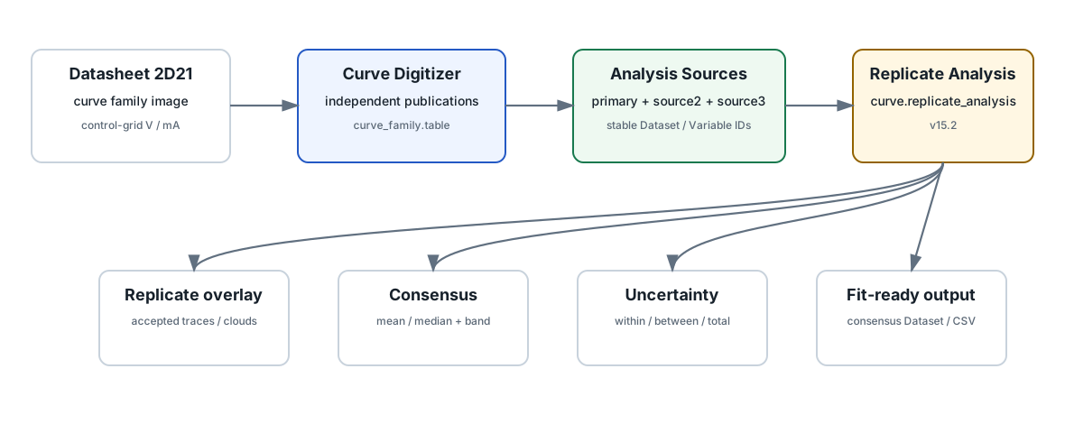
Workflow del caso di studio 2D21 — Dal datasheet alle pubblicazioni del Curve Digitizer, quindi alle Analysis Sources e ai risultati statistici.

1. La sorgente: una famiglia di curve nel datasheet

La sorgente è il grafico Average Grid Characteristics During Anode Conduction della 2D21 Sylvania. L'asse orizzontale rappresenta la tensione continua della control-grid; l'asse verticale la corrente continua della control-grid. Le curve sono parametrizzate dalla corrente anodica e comprendono i membri 25, 50, 100, 150, 200 e 300 mA.

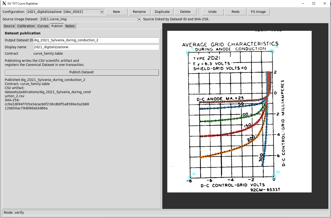
Curva 2D21 digitalizzata con GX-TXT Curve Digitizer — Il Curve Digitizer dopo calibrazione degli assi. I punti colorati ricostruiscono i diversi membri della famiglia direttamente dalla figura del datasheet.

Il punto importante non è soltanto ottenere una tabella numerica. Il digitizer pubblica un vero Dataset GX-TXT con contract curve_family.table, Dataset ID stabile e SHA-256 della sorgente collegata. In questo modo l'immagine originale, la calibrazione e il risultato numerico rimangono parte della provenance della Session.

2. Perché sono state fatte tre digitalizzazioni

Una digitalizzazione manuale non è una misura perfettamente deterministica. Il posizionamento del cursore, la densità dei punti, lo spessore della linea stampata e le zone quasi verticali del grafico introducono una variabilità osservabile. Ripetere la digitalizzazione consente di descrivere questa variabilità invece di nasconderla dentro una sola traccia.

Le tre pubblicazioni restano separate:

primary = dig_2D21_Sylvania_during_conduction_1
source2 = dig_2D21_Sylvania_during_conduction_2
source3 = dig_2D21_Sylvania_during_conduction_3

Questa scelta è importante: la separazione fra sorgenti permette al modulo di distinguere il comportamento interno alle ripetizioni dal disaccordo fra sorgenti, quando l'informazione disponibile rende identificabili le due componenti.

3. Configurazione della Session

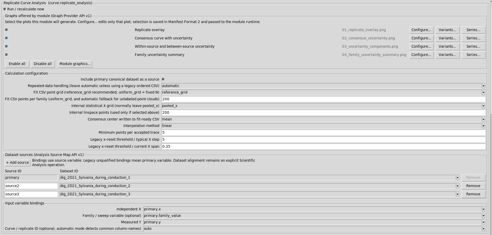
Replicate Curve Analysis configurato con tre Analysis Sources — Tre Dataset sorgente vengono associati allo stesso modulo senza fondere prematuramente i dati.

La configurazione mostrata usa automatic per il repeated-data handling, reference_grid per l'output fit-ready, pooled_x per la griglia statistica interna, media come centro del consenso e interpolazione lineare. I binding scientifici sono X, Family, Y e un replicate ID lasciato in automatico.

La variabile Family identifica il membro fisico della famiglia — per esempio 25 mA o 150 mA — mentre un eventuale Replicate ID identifica una ripetizione della stessa famiglia. Le due identità non sono intercambiabili.

4. Prima lettura: replicate overlay

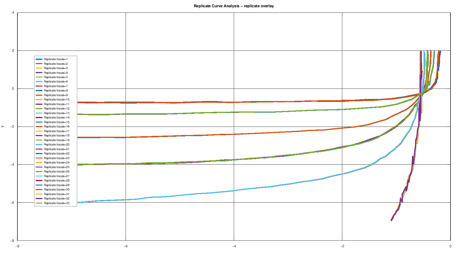
Replicate overlay della Session 2D21 — Le tracce accettate vengono sovrapposte prima di qualunque compressione statistica.

Questo è il grafico diagnostico iniziale. Permette di vedere immediatamente dove le digitalizzazioni concordano e dove divergono. Nel caso 2D21 la regione vicina alla conduzione più ripida è particolarmente sensibile: piccole differenze di posizione sull'immagine possono produrre differenze numeriche più evidenti.

L'overlay serve anche a verificare che le famiglie siano state interpretate correttamente, che nessuna sorgente sia accidentalmente scambiata per un'altra e che il dominio comune usato per il consenso abbia senso.

5. Dalle repliche alla curva di consenso

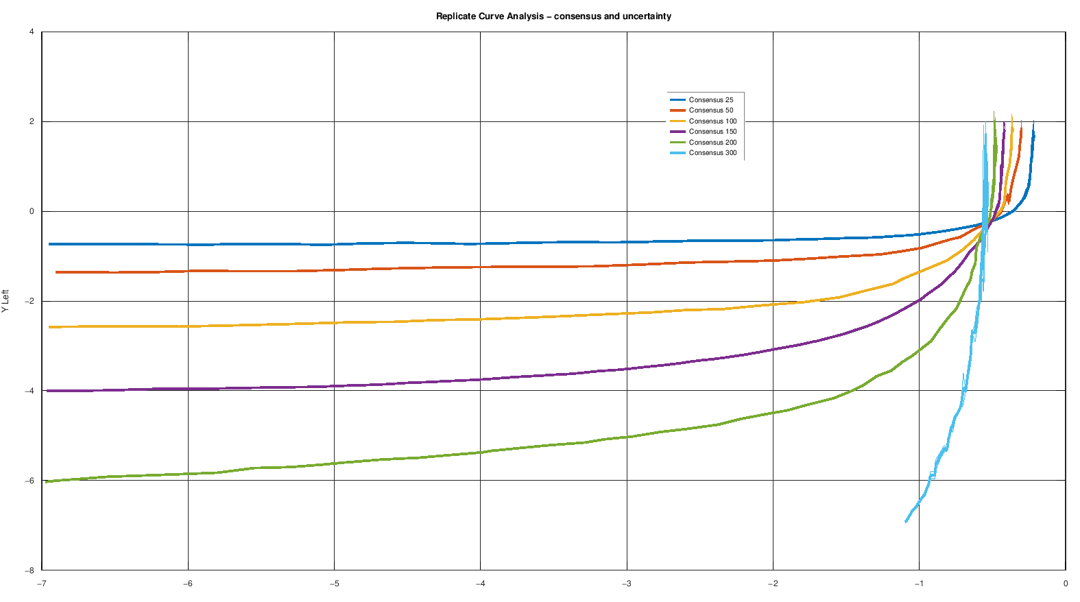
Curve di consenso e incertezza — Le ripetizioni vengono ridotte a una curva centrale per ciascun membro della famiglia, mantenendo l'informazione sulla dispersione.

La curva di consenso è ciò che consente di passare da più digitalizzazioni a un Dataset utilizzabile nei passaggi successivi. A seconda della configurazione la rappresentazione può essere accompagnata da dispersione, SEM o componente totale dell'incertezza, nei casi in cui quella quantità sia statisticamente definita.

Il risultato non va letto come “la curva vera” del dispositivo: è il consenso ottenuto dalle sorgenti incluse nella Session e secondo le scelte statistiche documentate nel run.

6. Dove nasce la dispersione

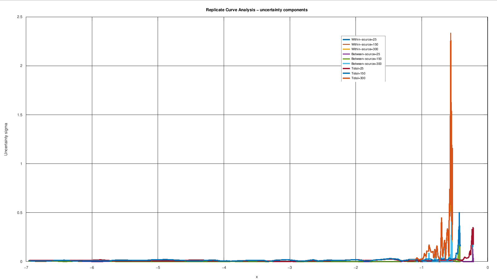
Componenti within-source, between-source e total — Le componenti vengono mostrate lungo X, permettendo di localizzare le regioni problematiche invece di ridurre subito tutto a un solo numero.

Quando identificabili, il modulo separa sigma_within, sigma_between e la loro combinazione sigma_total. Questo non attribuisce automaticamente una causa fisica: “between-source” significa soltanto che le sorgenti non concordano quanto ci si aspetterebbe dalla sola dispersione interna disponibile.

Nel contesto della digitalizzazione, una crescita localizzata dell'incertezza può essere coerente con una zona grafica difficile da leggere, ma questa interpretazione deve restare distinta dal risultato statistico prodotto dal modulo.

7. Confronto sintetico fra famiglie

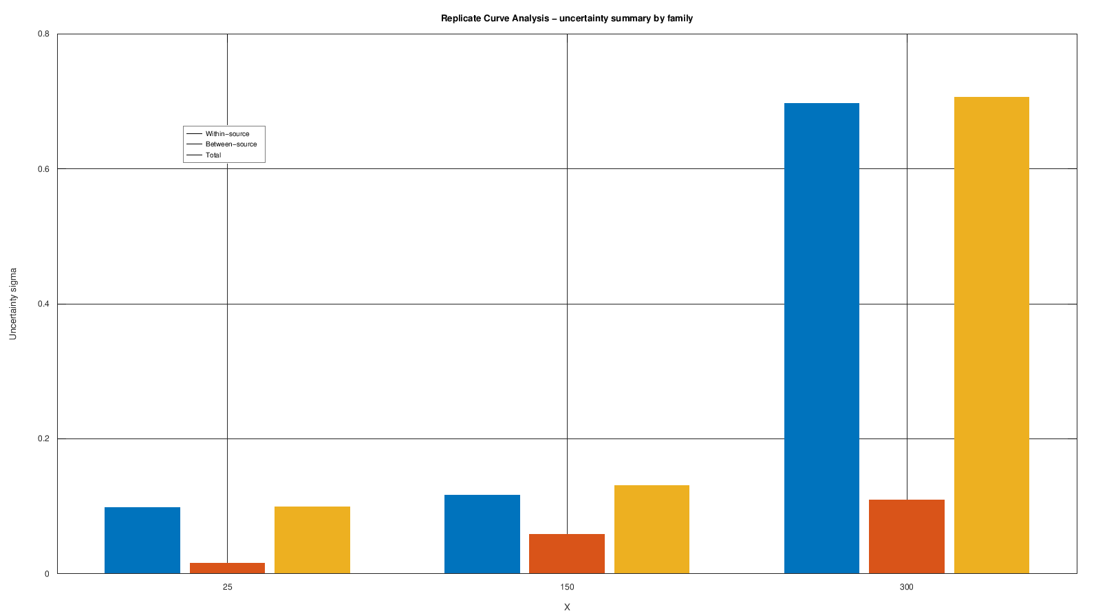
Riepilogo dell'incertezza per famiglia — Il family summary condensa i profili d'incertezza in valori scalari per confronto rapido.

Il riepilogo permette di confrontare rapidamente membri diversi della famiglia, ma è volutamente una compressione. Per capire dove una famiglia diventa instabile bisogna tornare al profilo completo dell'incertezza lungo X.

8. Il passaggio successivo: dati fit-ready

Il modulo produce anche un output destinato al fitting. Questo consente di non adattare direttamente un modello fisico a una nuvola di punti la cui densità dipende da quanti click sono stati fatti durante la digitalizzazione. Il fitting riceve invece una griglia controllata e una curva centrale derivata esplicitamente dalle repliche.

Da qui la Session può proseguire verso Curve fitting, mantenendo separati due problemi diversi:

quanto sono ripetibili e coerenti le curve di partenza;
quanto bene un modello fisico descrive il consenso ottenuto.

9. Cosa mostra questa Session di GX-TXT

una figura scientifica può diventare un Dataset canonico senza perdere provenance;
più digitalizzazioni possono restare sorgenti distinte invece di essere fuse manualmente;
Analysis Source Map permette a un modulo di lavorare su più Dataset contemporaneamente;
la statistica delle repliche viene separata dal successivo fitting fisico;
i grafici sono risultati persistenti e rerenderizzabili, non PNG isolati;
gli output derivati possono alimentare altri moduli della stessa Session.

Indice

1. What this module does

2. Scientific question answered by the module

3. Important non-goals

Part I — Input data model

4. Required bindings

5. The Family variable

6. The Replicate variable

7. Multiple Analysis Sources

8. Dataset access

Part II — Repeated-data modes

9. replicate_handling

10. Automatic mode

11. Automatic mode with explicit replicate IDs

12. Unlabelled repeated-point-cloud mode

13. one_curve_per_source_family

Important limitation

14. legacy_ordered_rows

Use this mode only when necessary

Part III — Input cleaning

15. Invalid rows

16. Minimum trace/cloud point count

17. Duplicate X values

Explicit traces

Unlabelled clouds

Part IV — Common X domain and interpolation

18. Why a common domain is required

19. Internal common-grid modes

20. pooled_x

21. linspace

22. Interpolation

Part V — Statistics with explicit repeated traces

23. Consensus curve

24. Pointwise sample standard deviation

25. Standard error

26. Source-based variance decomposition

27. When variance decomposition is identifiable

Identifiable

Not identifiable

Not identifiable

Part VI — Statistics for unlabelled point clouds

28. Why a different estimator is required

29. Local neighbourhood size

30. Local quadratic regression

31. Fallback for ill-conditioned local regression

32. Local residual dispersion

33. Combining several point-cloud sources

34. Why y_sem is unavailable for unlabelled clouds

35. Point-cloud mode with too few sources

Part VII — Fit-ready output grid

36. Why the fit output grid is separate

37. fit_output_grid

38. reference_grid

39. uniform_grid

40. Automatic fallback for unlabelled clouds

41. consensus_center

Part VIII — Configuration reference

42. include_primary_dataset

43. replicate_handling

44. min_trace_points

45. reset_step_factor

46. reset_span_fraction

47. common_grid

48. grid_points

49. fit_output_grid

50. fit_output_grid_points

51. interpolation

52. consensus_center

Part IX — Output files

53. consensus_for_fitting.csv

54. uncertainty_profile.csv

n

n_sources

statistics_mode

55. replicate_statistics.csv

source_path

representation

direction

56. source_statistics.csv

mean_bias

9. `replicate_handling`

13. `one_curve_per_source_family`

14. `legacy_ordered_rows`

20. `pooled_x`

21. `linspace`

34. Why `y_sem` is unavailable for unlabelled clouds

37. `fit_output_grid`

38. `reference_grid`

39. `uniform_grid`

41. `consensus_center`

42. `include_primary_dataset`

43. `replicate_handling`

44. `min_trace_points`

45. `reset_step_factor`

46. `reset_span_fraction`

47. `common_grid`

48. `grid_points`

49. `fit_output_grid`

50. `fit_output_grid_points`

51. `interpolation`

52. `consensus_center`

53. `consensus_for_fitting.csv`

54. `uncertainty_profile.csv`

`n`

`n_sources`

`statistics_mode`

55. `replicate_statistics.csv`

`source_path`

`representation`

`direction`

56. `source_statistics.csv`

`mean_bias`

`rms_deviation`

`max_abs_deviation`

57. `replicate_analysis_summary.txt`

58. `render_cache.mat`

59. `curve.replicate.traces`

60. `curve.replicate.profiles`

61. `curve.replicate.family_summary`

71. `y_std` band

72. `y_sem` band

73. `sigma_total` band

77. `sigma_within`

78. `sigma_between`

79. `sigma_total`