Indice
Workflow verificato GX-TXT dev-037 o successiva Tutorial Python
Questo tutorial mostra un workflow scientifico completo nel quale Python esegue il calcolo, ma GX-TXT conserva l'autorità su identità dei Dataset, metadata, provenance, pubblicazione, grafici e stato interattivo. Il risultato non è una figura Matplotlib o un file mesh privato: superficie, mesh e scena interattiva diventano normali oggetti persistenti della Session.
plot.dataset.xyz, crea un Interactive Document e conserva l'identità scientifica fino al Native 3D Viewer.Indice
- Materiali e risultato finale
- Architettura del workflow
- Dataset famiglia sorgente
- Metadata come parte del metodo
- Registrare gli script Python
- Stage 1 — fit e pubblicazione
- Teoria del fit polinomiale
- Dataset Publication e provenance
- Metadata del Dataset derivato
- Stage 2 — superficie 3D
- Nota sul bug trovato durante la prova
- Stage 3 — mesh e scena interattiva
- Native 3D Viewer
- Stage 4 — verifica dopo reopen
- Pattern riutilizzabili
- Checklist di riproduzione
- Download
1. Materiali e risultato finale
Il pacchetto del tutorial contiene il Dataset sorgente, metadata portabili e quattro script esattamente uguali a quelli usati nella prova.
| File | Ruolo |
|---|---|
terrain_profiles_raw.csv | 891 righe: 11 profili Y × 81 campioni X. |
terrain_profiles_raw.metadata.txt | Semantica, unità, binding, modello di fit, risoluzione della griglia e hint di presentazione. |
01_fit_publish_terrain.py | Legge il Dataset, esegue il fit polinomiale con NumPy, pubblica tutorial.terrain_surface_fit e scrive i metadata derivati. |
02_render_surface_v3.py | Crea e renderizza una normale Variant 3D surface tramite Plot Dataset v3. |
03_build_mesh_scene_v3.py | Crea la Variant mesh, chiama build_scene e verifica l'identità scientifica nella scena Native 3D. |
04_verify_after_reopen.py | Dopo chiusura e riapertura verifica metadata, Variant, rappresentazioni interattive e Interactive Documents persistenti. |
Con i dati forniti il fit produce circa RMSE = 0.575563 m e R² = 0.998712481; la griglia pubblicata è 81 × 51 = 4131 punti.
2. Architettura del workflow
terrain_profiles_raw.csv
        ↓ import
canonical family Dataset
        ↓
portable Dataset Metadata
        ↓
Python Script Workspace
01_fit_publish_terrain.py
        ↓ NumPy least squares
DATASET_PUBLICATION_API_v2
        ↓
tutorial.terrain_surface_fit
        ↓ DATASET_METADATA_API_v1/update
02_render_surface_v3.py
        ↓
plot.dataset.xyz / surface Variant
        ↓
03_build_mesh_scene_v3.py
        ↓
plot.dataset.xyz / mesh Variant
        ↓ PLOT_DATASET_API_v3/build_scene
Interactive Document
        ↓
Native 3D Viewer
        ↓ save / close / reopen
04_verify_after_reopen.py
Nessuno script modifica direttamente Manifest, Dataset Registry, file di persistenza di Plot Dataset o stato interno del Viewer.
3. Dataset famiglia sorgente
Il CSV usa cinque colonne:
| Colonna | Significato | Intervallo/struttura |
|---|---|---|
x_m | Coordinata X del profilo | 0…80 m, 81 valori |
y_m | Coordinata Y del profilo | 0…50 m, 11 valori |
z_m | Quota sintetica rumorosa | circa 178…262 m |
profile_id | Identità del membro della famiglia | 1…11 |
profile_y_m | Y associata al membro | una Y costante per ogni profile_id |
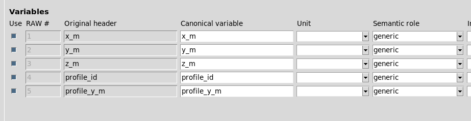
profile_id rappresenta una sezione a Y costante; X varia lungo il profilo. Lo script verifica esplicitamente questa semantica prima di adattare una superficie globale.4. Metadata come parte del metodo scientifico
Il file terrain_profiles_raw.metadata.txt non è una semplice descrizione. Contiene dati che determinano il comportamento dello script: nomi logici delle variabili, unità, numero atteso di profili, modello e grado del fit, densità della griglia di output e tipo di rappresentazione 3D.
Semantica e geometria
data.synthetic | true |
demo.type | python_script_terrain_flow |
demo.domain | synthetic_terrain |
terrain.coordinate_system | local_cartesian |
terrain.surface_quantity | elevation |
terrain.x_unit | m |
terrain.y_unit | m |
terrain.z_unit | m |
terrain.x_min_m | 0 |
terrain.x_max_m | 80 |
terrain.x_step_m | 1 |
terrain.y_min_m | 0 |
terrain.y_max_m | 50 |
terrain.profile_axis | y |
terrain.profile_count | 11 |
terrain.profile_points | 81 |
terrain.profile_spacing_m | 5 |
terrain.noise_sigma_m | 0.6 |
terrain.random_seed | 20261004 |
family.variable | profile_id |
family.coordinate_variable | profile_y_m |
Binding tra metadata e schema canonico
binding.x | x_m |
binding.y | y_m |
binding.z | z_m |
binding.family | profile_id |
Fit e presentazione
model.type | quartic_terrain_surface |
model.total_degree | 4 |
model.equation | z=180+0.30*u-0.22*v+0.018*u^2+0.030*v^2-0.016*u*v-0.00020*u^3+0.00015*u^2*v-0.00012*u*v^2+0.000006*u^4+0.000010*v^4-0.000005*u^2*v^2, u=x-40, v=y-25 |
fit.model | polynomial_total_degree |
fit.degree | 4 |
fit.grid_nx | 81 |
fit.grid_ny | 51 |
fit.output_dataset_id | tutorial.terrain_surface_fit |
presentation.surface_plot_type | surface |
presentation.mesh_plot_type | mesh |
interactive.target | native_3d |
5. Registrare gli script nel Python Script Workspace
Gli script sono registrati come risorse della Session, non eseguiti come file anonimi sparsi sul filesystem.
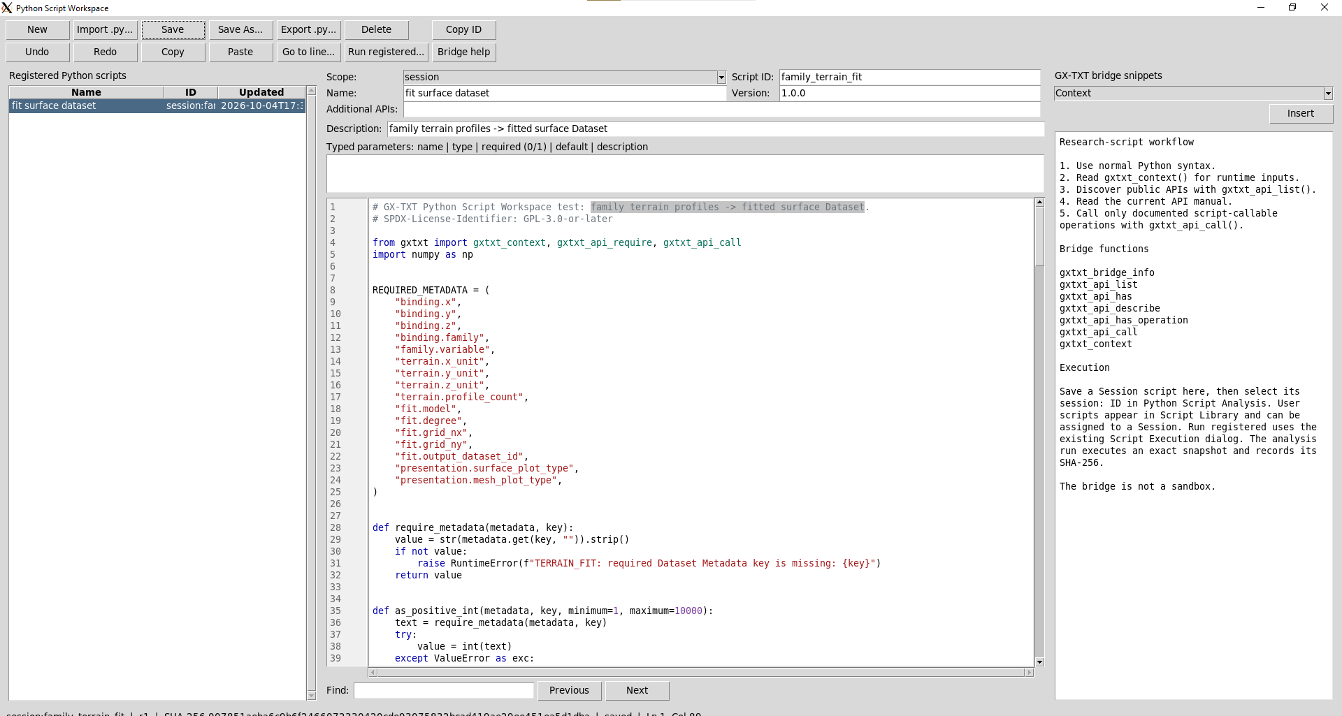
01_fit_publish_terrain.py nel Python Script Workspace.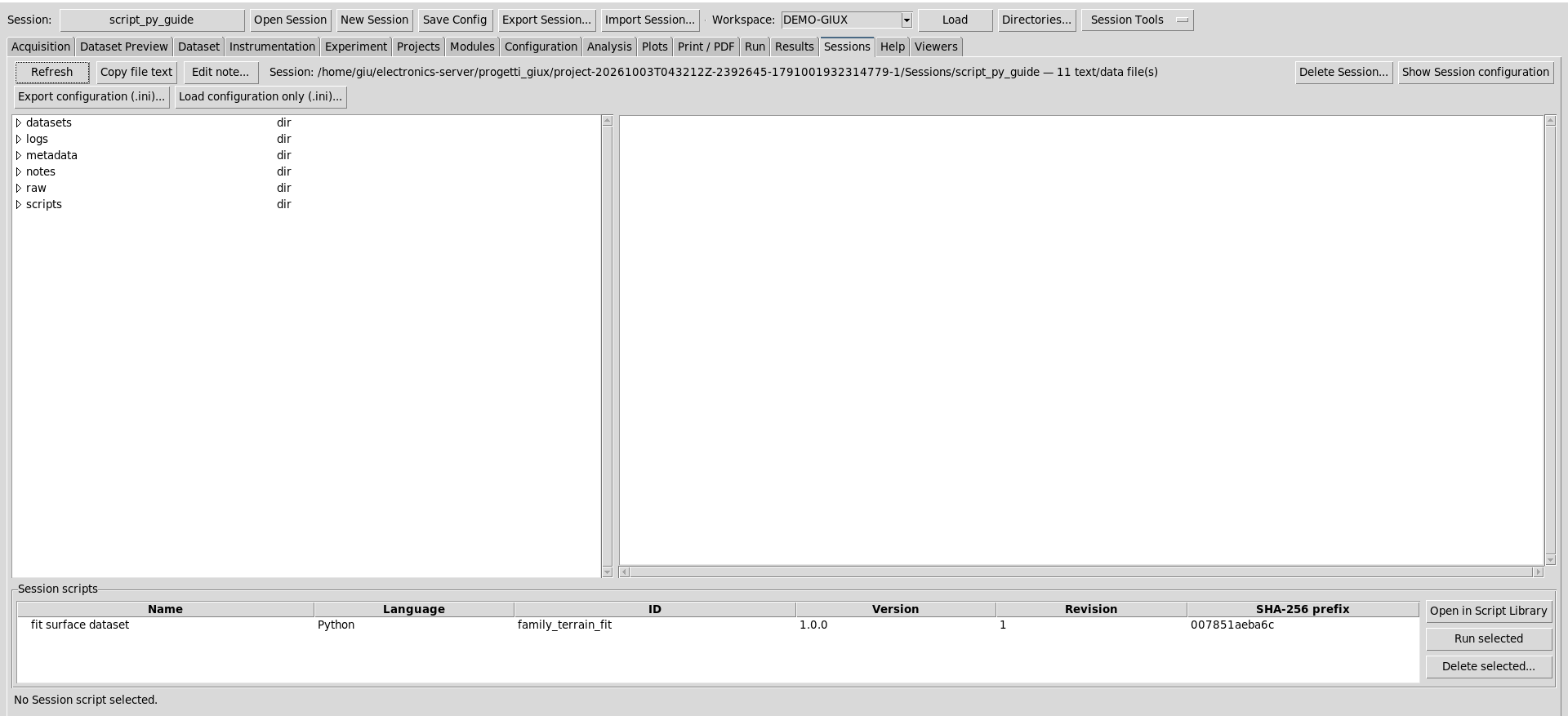
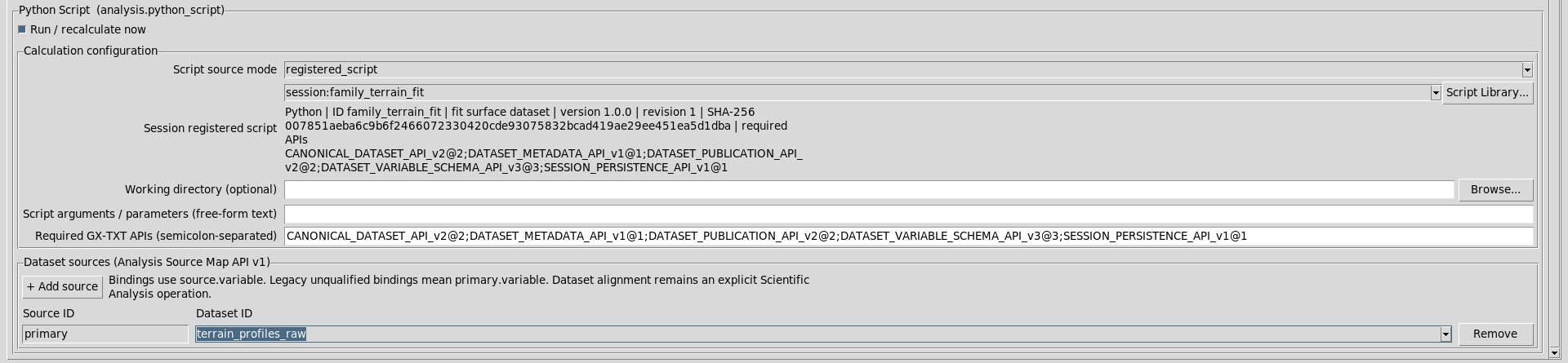
Per lo Stage 1 il Dataset raw viene assegnato come Analysis Source primary.
6. Stage 1 — leggere, adattare e pubblicare
01_fit_publish_terrain.py richiede in preflight:
CANONICAL_DATASET_API_v2DATASET_VARIABLE_SCHEMA_API_v3DATASET_METADATA_API_v1DATASET_PUBLICATION_API_v2SESSION_PERSISTENCE_API_v1
ctx = gxtxt_context()

gxtxt_api_require([
    "CANONICAL_DATASET_API_v2@2",
    "DATASET_VARIABLE_SCHEMA_API_v3@3",
    "DATASET_METADATA_API_v1@1",
    "DATASET_PUBLICATION_API_v2@2",
    "SESSION_PERSISTENCE_API_v1@1",
])

inputs = ctx.get("inputs", {})
primary = inputs.get("primary")
if not isinstance(primary, dict) or not primary.get("dataset_id"):
    raise RuntimeError("TERRAIN_FIT: select the raw terrain family Dataset as Analysis Source 'primary'")

source_dataset_id = str(primary["dataset_id"])
metadata = gxtxt_api_call("DATASET_METADATA_API_v1", "read", [source_dataset_id])

for key in REQUIRED_METADATA:
    require_metadata(metadata, key)

if require_metadata(metadata, "fit.model") != "polynomial_total_degree":
    raise RuntimeError("TERRAIN_FIT: this test requires fit.model=polynomial_total_degree")

degree = as_positive_int(metadata, "fit.degree", 1, 8)
grid_nx = as_positive_int(metadata, "fit.grid_nx", 2, 2000)
grid_ny = as_positive_int(metadata, "fit.grid_ny", 2, 2000)
expected_family_count = as_positive_int(metadata, "terrain.profile_count", 1, 10000)
output_dataset_id = require_metadata(metadata, "fit.output_dataset_id")
1Risolvere Variable ID stabili
I metadata contengono nomi logici come binding.x=x_m. Lo script confronta quei nomi con canonical, label, name e variable_id dello Schema v3 e ricava l'ID stabile da usare nelle successive API.
def resolve_variable_id(schema, requested_name):
    requested = requested_name.strip()
    for item in schema:
        candidates = []
        for field in ("canonical", "label", "name", "variable_id"):
            value = item.get(field)
            if value is not None:
                candidates.append(str(value).strip())
        if requested in candidates:
            return str(item["variable_id"])
    raise RuntimeError(
        f"TERRAIN_FIT: metadata requested variable {requested!r}, "
"but it is not present in the canonical Variable Schema"2Leggere i dati canonici
schema = gxtxt_api_call("DATASET_VARIABLE_SCHEMA_API_v3", "list", [source_dataset_id])

x_id = resolve_variable_id(schema, require_metadata(metadata, "binding.x"))
y_id = resolve_variable_id(schema, require_metadata(metadata, "binding.y"))
z_id = resolve_variable_id(schema, require_metadata(metadata, "binding.z"))
family_id = resolve_variable_id(schema, require_metadata(metadata, "binding.family"))

description = gxtxt_api_call("CANONICAL_DATASET_API_v2", "describe", [source_dataset_id])
row_count = int(description["row_count"])
if row_count < 16:
    raise RuntimeError("TERRAIN_FIT: source Dataset has too few rows")

block = gxtxt_api_call(
    "CANONICAL_DATASET_API_v2",
    "read_range",
    [source_dataset_id, [x_id, y_id, z_id, family_id], 0, row_count],
)

x = np.asarray(block[x_id]["values"], dtype=float).reshape(-1)
y = np.asarray(block[y_id]["values"], dtype=float).reshape(-1)
z = np.asarray(block[z_id]["values"], dtype=float).reshape(-1)
Il codice verifica allineamento delle righe, valori finiti e la relazione famiglia → Y costante prima del fit.
7. Teoria: fit polinomiale totale Z = f(X,Y)
Il modello usa un polinomio di grado totale d. Con coordinate normalizzate xn, yn include tutti i monomi:
\[x_n^{p_x} y_n^{p_y},\qquad p_x+p_y\le d.\]
Il numero di termini è:
\[N_{terms}= rac{(d+1)(d+2)}2.\]
Per d=4 si ottengono 15 coefficienti.
La normalizzazione usata dallo script è:
\[x_n= rac{x-x_c}{x_s},\qquad y_n= rac{y-y_c}{y_s},\]
con centro nel punto medio dell'intervallo e scala pari alla semiampiezza. Questo riduce la differenza di scala tra potenze di X e Y rispetto a una base costruita direttamente sulle coordinate 0…80 e 0…50.
Il problema di minimi quadrati è:
\[\min_c\|Ac-z\|_2.\]
x_min, x_max = float(np.min(x)), float(np.max(x))
y_min, y_max = float(np.min(y)), float(np.max(y))
x_center = 0.5 * (x_min + x_max)
y_center = 0.5 * (y_min + y_max)
x_scale = 0.5 * (x_max - x_min)
y_scale = 0.5 * (y_max - y_min)
if x_scale <= 0.0 or y_scale <= 0.0:
    raise RuntimeError("TERRAIN_FIT: X and Y must both span nonzero ranges")

xn = (x - x_center) / x_scale
yn = (y - y_center) / y_scale

powers = total_degree_powers(degree)
A = design_matrix(xn, yn, powers)
coefficients, _, rank, _ = np.linalg.lstsq(A, z, rcond=None)
if int(rank) != len(powers):
    raise RuntimeError(
        f"TERRAIN_FIT: polynomial design matrix rank {rank} is below {len(powers)}"
    )

z_fit_source = A @ coefficients
residual = z - z_fit_source
rmse = float(np.sqrt(np.mean(residual ** 2)))
ss_res = float(np.sum(residual ** 2))
ss_tot = float(np.sum((z - np.mean(z)) ** 2))
r2 = float(1.0 - ss_res / ss_tot) if ss_tot > 0.0 else 1.0

x_grid = np.linspace(x_min, x_max, grid_nx)
y_grid = np.linspace(y_min, y_max, grid_ny)
Xg, Yg = np.meshgrid(x_grid, y_grid, indexing="xy")
xgn = (Xg.reshape(-1) - x_center) / x_scale
ygn = (Yg.reshape(-1) - y_center) / y_scale
Ag = design_matrix(xgn, ygn, powers)
zg = Ag @ coefficients
Con il CSV fornito la matrice ha rango 15/15, RMSE ≈ 0.5755626 m e R² ≈ 0.99871248. La superficie viene poi valutata sulla griglia 81×51 indicata nei metadata.
8. Pubblicare il risultato come Dataset canonico
Lo script non salva semplicemente un CSV nella directory di lavoro. Apre un writer della Publication API, dichiara una dimensione row estendibile, dichiara X/Y/Z con unità e ruoli semantici, esegue un append allineato e finalizza la transazione.
definition = {
    "dataset_id": output_dataset_id,
    "contract": "table.generic",
    "storage": "auto",
    "replace_owned": True,
    "producer_version": "1.0.0",
    "source_dataset_ids": [source_dataset_id],
    "source_variable_ids": [x_id, y_id, z_id, family_id],
    "source": "Python Script Workspace terrain surface fit",
    "provenance": (
        f"Total-degree {degree} polynomial least-squares fit of Z=f(X,Y) "
        "from a family of terrain profiles."
    ),
    "notes": (
        "Dense rectangular fitted terrain grid. Fit settings and diagnostics "
        "are stored through Dataset Metadata API v1."
    ),
}

writer = gxtxt_api_call("DATASET_PUBLICATION_API_v2", "begin", [definition])
try:
    gxtxt_api_call(
        "DATASET_PUBLICATION_API_v2",
        "declare_dimension",
        [writer, "row", 0, {"extendible": 1}],
    )

    variable_definitions = (
        ("v_x_m", x_unit, "coordinate", "independent"),
        ("v_y_m", y_unit, "coordinate", "independent"),
        ("v_z_fit_m", z_unit, "data", "derived"),
    )
    for variable_id, unit, coordinate_role, semantic_role in variable_definitions:
        schema_def = {
            "dtype": "float64",
            "rank": 1,
            "dimension_ids": "row",
            "coordinate_role": coordinate_role,
            "semantic_role": semantic_role,
            "unit": unit,
        }
        gxtxt_api_call(
            "DATASET_PUBLICATION_API_v2",
            "declare_variable",
            [writer, variable_id, schema_def],
        )

    gxtxt_api_call(
        "DATASET_PUBLICATION_API_v2",
        "append",
        [
            writer,
            "row",
            {
                "v_x_m": out_x,
                "v_y_m": out_y,
                "v_z_fit_m": out_z,
            },
        ],
    )

    published = gxtxt_api_call("DATASET_PUBLICATION_API_v2", "finalize", [writer])
L'output stabile è:
Dataset ID: tutorial.terrain_surface_fit
Contract:   table.generic
Variables:  v_x_m, v_y_m, v_z_fit_m
Rows:       4131
9. Metadata del Dataset derivato
Dopo la pubblicazione, lo script salva sul nuovo Dataset sia provenance e diagnostica del fit, sia gli ID variabile necessari ai passaggi successivi.
derived_metadata = {
    "data.synthetic": str(metadata.get("data.synthetic", "true")),
    "demo.type": "python_script_terrain_fit_output",
    "demo.domain": str(metadata.get("demo.domain", "synthetic_terrain")),
    "terrain.coordinate_system": str(metadata.get("terrain.coordinate_system", "local_cartesian")),
    "terrain.surface_quantity": str(metadata.get("terrain.surface_quantity", "elevation")),
    "terrain.x_unit": x_unit,
    "terrain.y_unit": y_unit,
    "terrain.z_unit": z_unit,
    "terrain.grid_nx": str(grid_nx),
    "terrain.grid_ny": str(grid_ny),
    "terrain.grid_rows": str(grid_nx * grid_ny),
    "processing.kind": "surface_fit",
    "processing.language": "python",
    "processing.source_dataset_id": source_dataset_id,
    "processing.source_family_variable_id": family_id,
    "processing.source_family_count": str(family_members.size),
    "fit.model": "polynomial_total_degree",
    "fit.degree": str(degree),
    "fit.basis": "normalized_xy_total_degree",
    "fit.term_powers": power_text,
    "fit.coefficients": coefficient_text,
    "fit.x_center": f"{x_center:.17g}",
    "fit.x_scale": f"{x_scale:.17g}",
    "fit.y_center": f"{y_center:.17g}",
    "fit.y_scale": f"{y_scale:.17g}",
    "fit.rmse_m": f"{rmse:.17g}",
    "fit.r2": f"{r2:.17g}",
    "schema.x_variable_id": "v_x_m",
    "schema.y_variable_id": "v_y_m",
    "schema.z_variable_id": "v_z_fit_m",
    "presentation.surface_plot_type": require_metadata(metadata, "presentation.surface_plot_type"),
    "presentation.mesh_plot_type": require_metadata(metadata, "presentation.mesh_plot_type"),
    "interactive.target": str(metadata.get("interactive.target", "native_3d")),
}

updated_metadata = gxtxt_api_call(
    "DATASET_METADATA_API_v1",
    "update",
    [output_dataset_id, derived_metadata],
)

gxtxt_api_call("SESSION_PERSISTENCE_API_v1", "commit", [])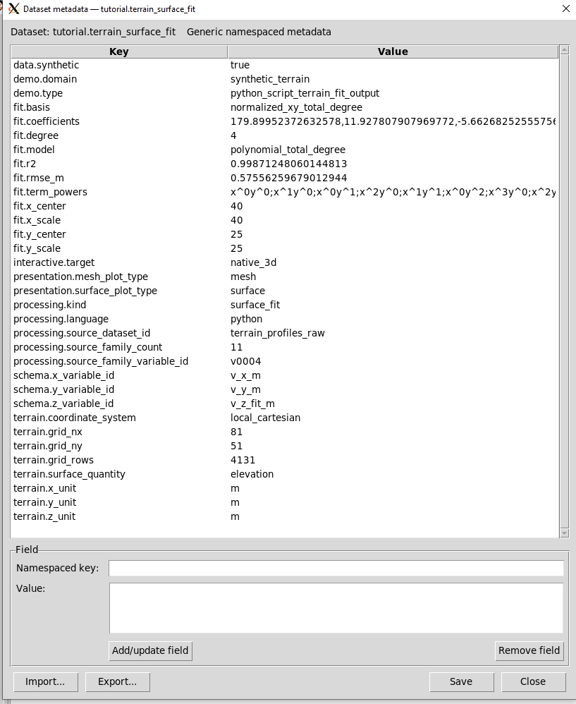
v_x_m, v_y_m, v_z_fit_m o decidere autonomamente se usare surface o mesh. Leggono questi valori dal risultato scientifico appena pubblicato.10. Stage 2 — creare una normale superficie 3D Plot Dataset
02_render_surface_v3.py usa come primary il Dataset derivato.
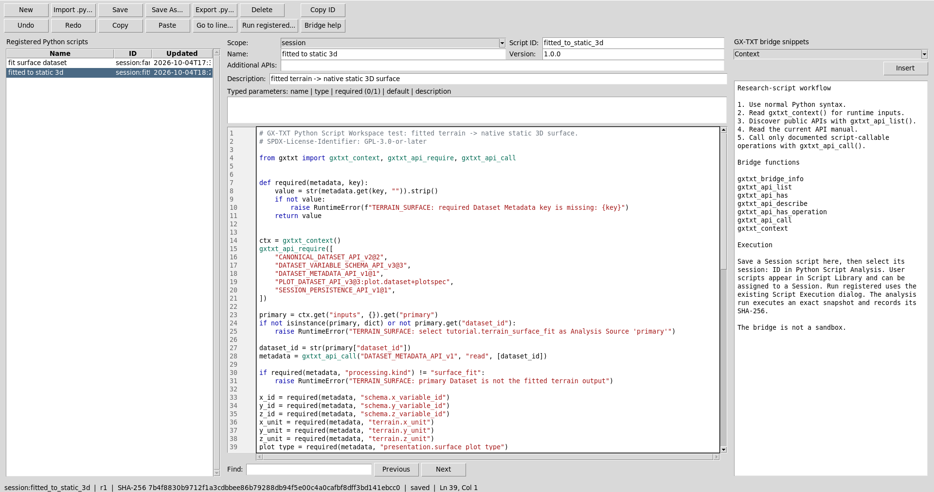
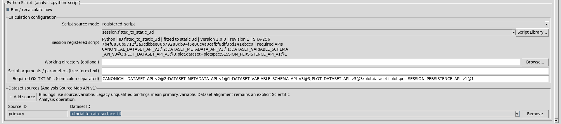
Lo script legge i Variable ID e le unità dai metadata, costruisce un PlotSpec cartesian_3d con graph_id=plot.dataset.xyz e plot_type=surface, lo valida, crea una Variant normale e la renderizza.
dataset_id = str(primary["dataset_id"])
metadata = gxtxt_api_call("DATASET_METADATA_API_v1", "read", [dataset_id])

if required(metadata, "processing.kind") != "surface_fit":
    raise RuntimeError("TERRAIN_SURFACE: primary Dataset is not the fitted terrain output")

x_id = required(metadata, "schema.x_variable_id")
y_id = required(metadata, "schema.y_variable_id")
z_id = required(metadata, "schema.z_variable_id")
x_unit = required(metadata, "terrain.x_unit")
y_unit = required(metadata, "terrain.y_unit")
z_unit = required(metadata, "terrain.z_unit")
plot_type = required(metadata, "presentation.surface_plot_type")

if plot_type != "surface":
    raise RuntimeError(
        f"TERRAIN_SURFACE: metadata presentation.surface_plot_type must be 'surface', got {plot_type!r}"
    )

# Verify that the metadata-carried stable IDs still exist in the canonical schema.
for variable_id in (x_id, y_id, z_id):
    gxtxt_api_call("DATASET_VARIABLE_SCHEMA_API_v3", "get", [dataset_id, variable_id])

description = gxtxt_api_call("CANONICAL_DATASET_API_v2", "describe", [dataset_id])
if int(description["row_count"]) < 4:
    raise RuntimeError("TERRAIN_SURFACE: fitted Dataset is empty or too small")

spec = {
    "schema": "PLOT_DATASET_PLOTSPEC_v2",
    "graph_type": "cartesian_3d",
    "graph_id": "plot.dataset.xyz",
    "dataset_id": dataset_id,
    "x_variable_id": x_id,
    "y_variable_id": y_id,
    "z_variable_id": z_id,
    "title": "Python fitted synthetic terrain",
    "config": {
        "plot_type": plot_type,
        "reduction_mode": "none",
        "x_label": f"X [{x_unit}]",
        "y_label": f"Y [{y_unit}]",
        "z_label": f"Elevation [{z_unit}]",
    },
}

if not gxtxt_api_call("PLOT_DATASET_API_v3", "validate_spec", [spec]):
    raise RuntimeError("TERRAIN_SURFACE: PlotSpec validation returned false")

plot_ref = gxtxt_api_call(
    "PLOT_DATASET_API_v3",
    "create_plot",
    [spec, "variant"],
)

render_result = gxtxt_api_call("PLOT_DATASET_API_v3", "render", [plot_ref])
artifacts = gxtxt_api_call("PLOT_DATASET_API_v3", "artifacts", [plot_ref])
gxtxt_api_call("SESSION_PERSISTENCE_API_v1", "commit", [])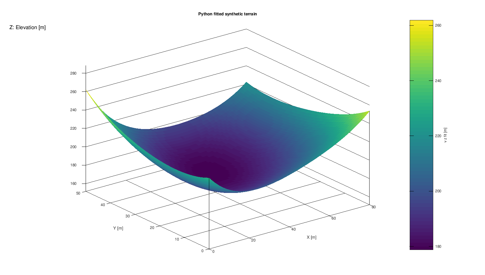
11. Nota storica: il bug emerso durante la validazione

validate_spec per il ramo cartesian_3d.true; PlotSpec non valido → errore esplicito. La correzione è stata fatta nel framework, non aggirata nello script. Il tutorial conserva questo episodio perché mostra il valore di un test end-to-end che usa davvero l'API pubblica.12. Stage 3 — mesh Plot Dataset e Interactive Document
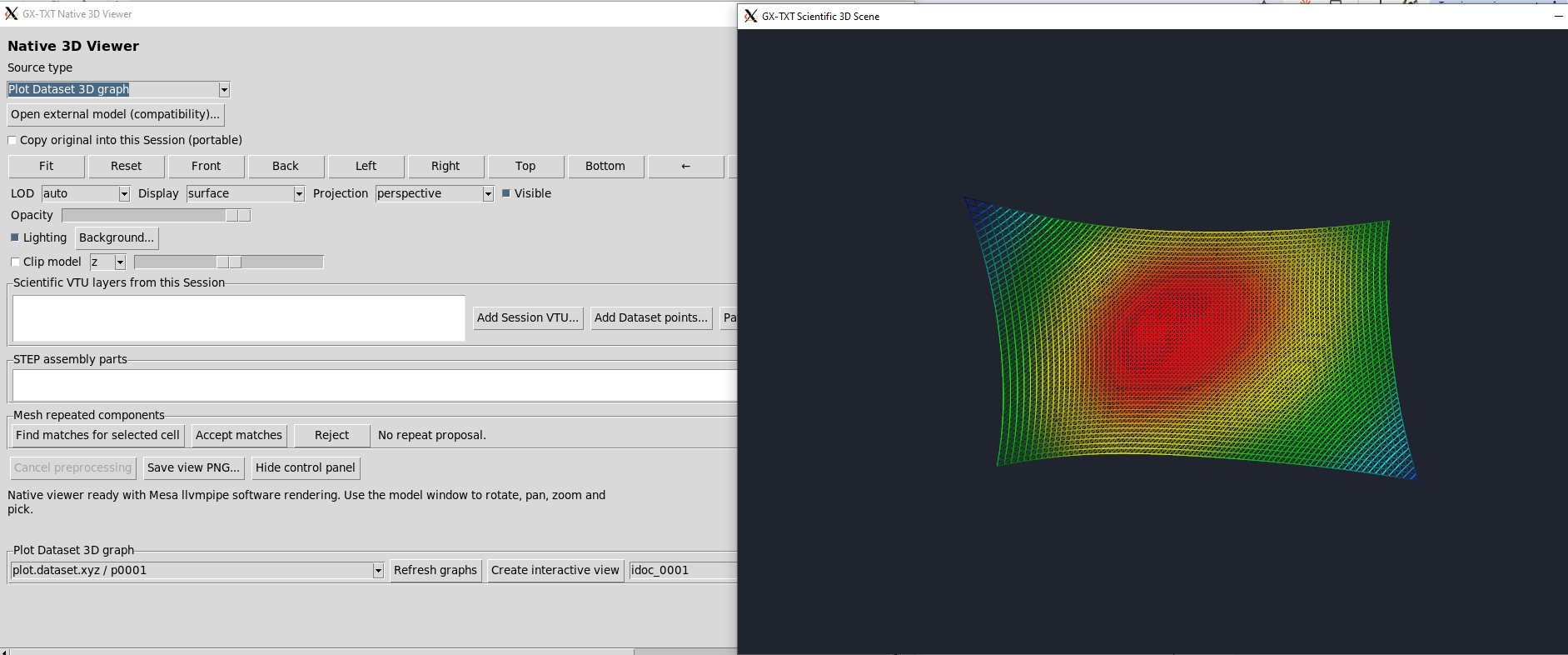
03_build_mesh_scene_v3.py parte ancora da tutorial.terrain_surface_fit, ma legge presentation.mesh_plot_type=mesh. Crea quindi una seconda Variant plot.dataset.xyz.
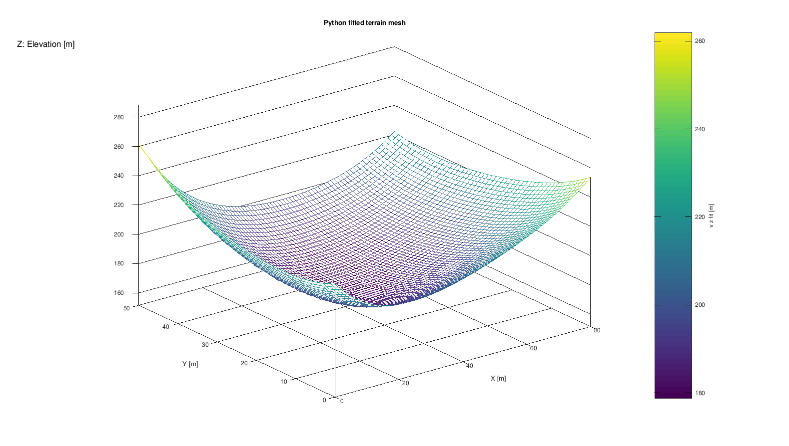
Dopo il render, la parte decisiva è build_scene:
if not gxtxt_api_call("PLOT_DATASET_API_v3", "validate_spec", [spec]):
    raise RuntimeError("TERRAIN_MESH: PlotSpec validation returned false")

mesh_ref = gxtxt_api_call(
    "PLOT_DATASET_API_v3",
    "create_plot",
    [spec, "variant"],
)

gxtxt_api_call("PLOT_DATASET_API_v3", "render", [mesh_ref])
artifacts = gxtxt_api_call("PLOT_DATASET_API_v3", "artifacts", [mesh_ref])

scene = gxtxt_api_call("PLOT_DATASET_API_v3", "build_scene", [mesh_ref])
representation_id = str(scene["representation_id"])

status = gxtxt_api_call(
    "PLOT_DATASET_API_v3",
    "interactive_status",
    [representation_id],
)
if str(status) != "SYNCED":
    raise RuntimeError(
        f"TERRAIN_MESH: new interactive representation is not SYNCED: {status!r}"
    )

representations = gxtxt_api_call(
    "PLOT_DATASET_API_v3",
    "interactive_representations",
    [],
)
if not any(str(item.get("id", "")) == representation_id for item in representations):
    raise RuntimeError("TERRAIN_MESH: representation is missing from Plot Dataset interactive registry")

documents = gxtxt_api_call("INTERACTIVE_DOCUMENT_API_v1", "list", [])
if not any(str(item.get("id", "")) == representation_id for item in documents):
    raise RuntimeError("TERRAIN_MESH: representation is missing from Interactive Document registry")

viewer_identity = gxtxt_api_call("NATIVE_3D_VIEWER_API_v1", "source_identity", [])
layers = viewer_identity.get("layers", {})
if not layers:
    raise RuntimeError("TERRAIN_MESH: Native 3D scene contains no scientific layers")

matching_layers = 0
for layer in layers.values():
    if str(layer.get("source_dataset_id", "")) == dataset_id:
        matching_layers += 1
if matching_layers < 1:
    raise RuntimeError(
        "TERRAIN_MESH: Native 3D scene layers do not retain the fitted Dataset identity"
    )

gxtxt_api_call("SESSION_PERSISTENCE_API_v1", "commit", [])

print(
    "PASS TERRAIN_MESH_SCENE_V3 "
    f"dataset={dataset_id} graph={mesh_ref['graph_id']} "
    f"variant={mesh_ref['variant_id']} representation={representation_id} "
    f"status={status} layers={len(layers)} matching_source_layers={matching_layers} "
    f"artifact={artifacts.get('graph_artifact', '')}"
Il codice verifica tre livelli diversi di persistenza:
| Oggetto | Verifica |
|---|---|
| Plot Dataset representation | interactive_status deve essere SYNCED e l'ID deve comparire in interactive_representations. |
| Interactive Document | Lo stesso representation ID deve comparire in INTERACTIVE_DOCUMENT_API_v1/list. |
| Native 3D scene | Almeno un layer restituito da NATIVE_3D_VIEWER_API_v1/source_identity deve conservare source_dataset_id=tutorial.terrain_surface_fit. |
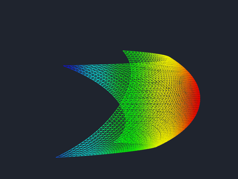
13. Native 3D Viewer: la scena è realmente interattiva
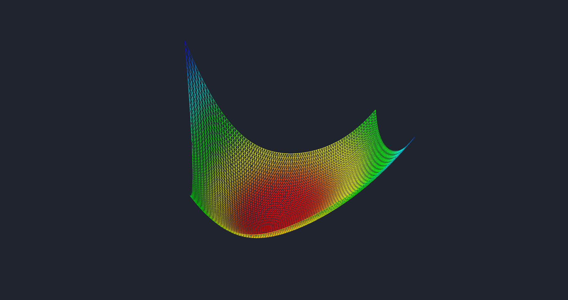
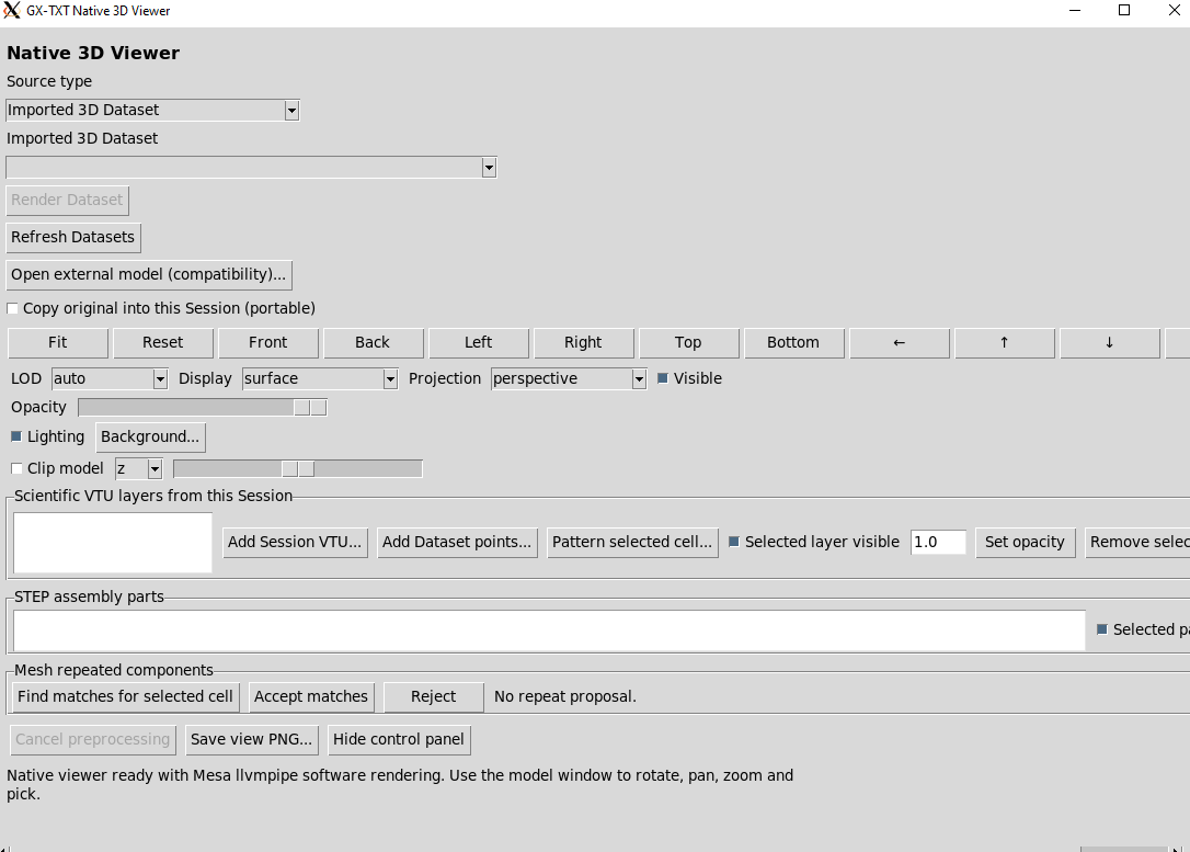
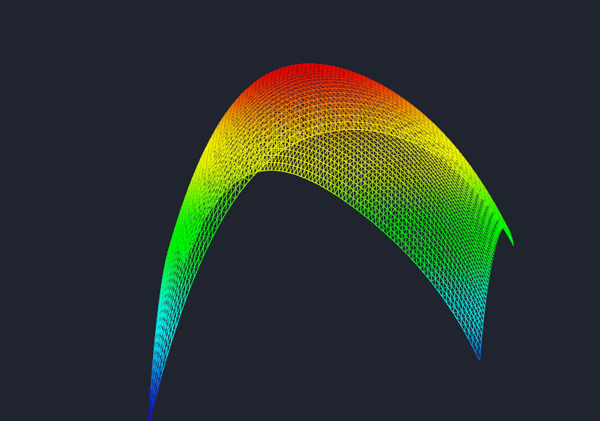

persistent plot.dataset.xyz Variant
        ↓ build_scene
scientific VTP representation + provenance
        ↓
Interactive Document
        ↓
GX-TXT Native 3D scientific scene
14. Stage 4 — chiudere, riaprire e verificare
Il quarto script va eseguito dopo aver chiuso e riaperto la Session. Non ricrea gli oggetti: controlla che ciò che dovrebbe essere persistente sia ancora presente.
ctx = gxtxt_context()
gxtxt_api_require([
    "CANONICAL_DATASET_API_v2@2",
    "DATASET_METADATA_API_v1@1",
    "PLOT_MODULE_API_v1@1",
    "PLOT_DATASET_API_v3@3:plot.dataset+plotspec",
    "INTERACTIVE_DOCUMENT_API_v1@1",
])

primary = ctx.get("inputs", {}).get("primary")
if not isinstance(primary, dict) or not primary.get("dataset_id"):
    raise RuntimeError("TERRAIN_VERIFY: select tutorial.terrain_surface_fit as Analysis Source 'primary'")

dataset_id = str(primary["dataset_id"])
metadata = gxtxt_api_call("DATASET_METADATA_API_v1", "read", [dataset_id])

required_keys = (
    "processing.kind",
    "processing.source_dataset_id",
    "fit.model",
    "fit.degree",
    "fit.rmse_m",
    "fit.r2",
    "schema.x_variable_id",
    "schema.y_variable_id",
    "schema.z_variable_id",
    "presentation.surface_plot_type",
    "presentation.mesh_plot_type",
)
missing = [key for key in required_keys if not str(metadata.get(key, "")).strip()]
if missing:
    raise RuntimeError(
        "TERRAIN_VERIFY: derived Dataset Metadata did not survive reopen: "
        + ", ".join(missing)
    )

dataset_description = gxtxt_api_call("CANONICAL_DATASET_API_v2", "describe", [dataset_id])
variant_ids = gxtxt_api_call(
    "PLOT_MODULE_API_v1",
    "variant_ids",
    ["plot.dataset", "plot.dataset.xyz"],
)

plot_types = {}
for variant_id in variant_ids:
    ref = gxtxt_api_call(
        "PLOT_DATASET_API_v3",
        "open_plot",
        ["plot.dataset.xyz", str(variant_id)],
    )
    state = gxtxt_api_call("PLOT_DATASET_API_v3", "read_plot", [ref])
    config = state.get("config", {}) if isinstance(state, dict) else {}
    plot_types[str(variant_id)] = str(config.get("plot_type", ""))

representations = gxtxt_api_call(
    "PLOT_DATASET_API_v3",
    "interactive_representations",
    [],
)
documents = gxtxt_api_call("INTERACTIVE_DOCUMENT_API_v1", "list", [])

if not variant_ids:
    raise RuntimeError("TERRAIN_VERIFY: no persistent plot.dataset.xyz Variants survived reopen")
if not representations:
    raise RuntimeError("TERRAIN_VERIFY: no persistent Plot Dataset interactive representations survived reopen")
if not documents:
    raise RuntimeError("TERRAIN_VERIFY: no Interactive Documents survived reopen")

print(
    "PASS TERRAIN_PERSISTENCE_VERIFY "
    f"dataset={dataset_id} rows={int(dataset_description['row_count'])} "
    f"metadata_keys={len(metadata)} xyz_variants={len(variant_ids)} "
    f"plot_types={plot_types} interactive_representations={len(representations)} "
    f"interactive_documents={len(documents)}"
La verifica copre:
- metadata del Dataset derivato;
- Dataset ancora descrivibile attraverso Canonical Dataset API;
- Variant
plot.dataset.xyzpersistenti; - configurazione
surface/meshleggibile dai grafici; - rappresentazioni interattive persistenti;
- Interactive Documents persistenti.
15. Cosa è specifico del terreno e cosa è riutilizzabile
| Specifico di questo tutorial | Pattern riutilizzabile |
|---|---|
| Famiglia di profili a Y costante | Usare metadata + Variable Schema per risolvere la semantica dei dati. |
| Fit polinomiale totale di grado 4 | Usare NumPy/SciPy per il calcolo senza sottrarre a GX-TXT la gestione dei dati. |
| Griglia 81×51 | Pubblicare il risultato mediante DATASET_PUBLICATION_API_v2. |
plot_type=surface e mesh | Creare grafici normali via PlotSpec + PLOT_DATASET_API_v3. |
| Terreno sintetico | Portare provenance, unità e binding nel Dataset derivato. |
| Native 3D come destinazione | Costruire una rappresentazione interattiva mantenendo l'identità del Dataset sorgente. |
16. API esercitate
| API | Uso |
|---|---|
CANONICAL_DATASET_API_v2 | Descrizione e lettura del Dataset canonico. |
DATASET_VARIABLE_SCHEMA_API_v3 | Risoluzione e verifica degli ID variabile stabili. |
DATASET_METADATA_API_v1 | Configurazione scientifica in ingresso e metadata/provenance derivati. |
DATASET_PUBLICATION_API_v2 | Writer transazionale per il Dataset della superficie adattata. |
PLOT_DATASET_API_v3 | Validate, create, render, artifacts, build_scene e stato delle rappresentazioni interattive. |
INTERACTIVE_DOCUMENT_API_v1 | Verifica dell'oggetto persistente che rappresenta la vista interattiva. |
NATIVE_3D_VIEWER_API_v1 | Verifica dell'identità scientifica dei layer della scena. |
SESSION_PERSISTENCE_API_v1 | Commit esplicito dello stato persistente. |
PLOT_MODULE_API_v1 | Nello script di reopen: enumerazione delle Variant persistenti. |
17. Checklist di riproduzione
Stage A — sorgente
- Importa
terrain_profiles_raw.csv. - Apri Dataset Metadata, importa
terrain_profiles_raw.metadata.txt, controlla e salva. - Verifica 891 righe e 11 famiglie.
Stage B — fit
- Registra
01_fit_publish_terrain.pycome Session script. - Seleziona il Dataset raw come
primary. - Esegui e verifica
PASS TERRAIN_FIT_PUBLISH. - Apri
tutorial.terrain_surface_fit, verifica 4131 righe e i metadatafit.*.
Stage C — superficie
- Registra
02_render_surface_v3.py. - Seleziona
tutorial.terrain_surface_fitcomeprimary. - Esegui e verifica
PASS TERRAIN_SURFACE_V3. - Controlla che la Variant compaia normalmente nella pagina Plots.
Stage D — mesh e scena
- Registra
03_build_mesh_scene_v3.py. - Mantieni il Dataset derivato come
primary. - Esegui e verifica
PASS TERRAIN_MESH_SCENE_V3. - Apri Native 3D e ispeziona la scena.
Stage E — persistenza
- Salva, chiudi e riapri la Session.
- Registra/esegui
04_verify_after_reopen.py. - Verifica
PASS TERRAIN_PERSISTENCE_VERIFY.
18. Download dei materiali
I file sono quelli originali forniti con la prova; gli script non sono stati riscritti per la documentazione.
19. Risultato
Il tutorial dimostra un principio generale: Python può essere il motore del calcolo senza diventare un sottosistema parallelo a GX-TXT. Le librerie scientifiche elaborano i numeri; il framework continua a governare Dataset, schema, metadata, provenance, grafici, interactive state e riapertura della Session.