Indice
Il workflow del demo
Il generator surface3d_thermal_field costruisce un campo termico sintetico e deterministico. Il plugin demo.visualization.surface3d 1.0.3 valida la struttura rettangolare X/Y/Z, calcola le metriche del campo e genera tre rappresentazioni complementari mediante il normale stack 3D di GX-TXT.
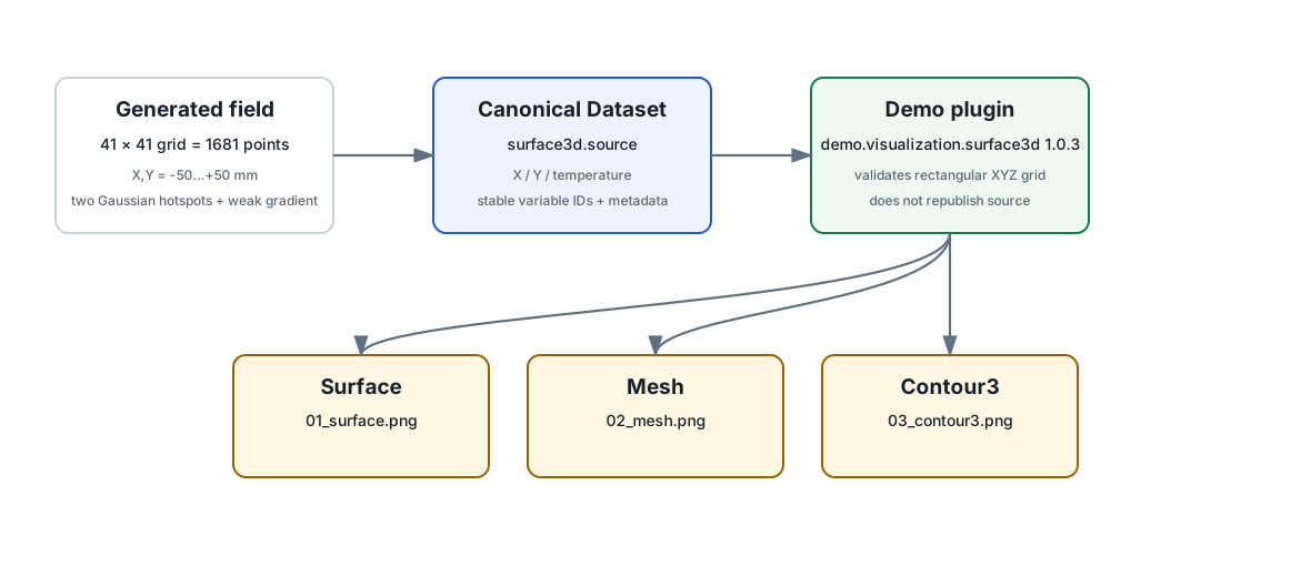
Il campo termico
La superficie copre un'area da −50 a +50 mm sia in X sia in Y, campionata su una griglia 41 × 41 con passo 2,5 mm: in totale 1681 punti. La temperatura è generata da due hotspot gaussiani sovrapposti a un debole gradiente lineare.
T(x,y) = 293.15
       + 18 exp(-((x+12)^2/(2·9^2)  + (y-8)^2/(2·12^2)))
       + 11 exp(-((x-16)^2/(2·14^2) + (y+10)^2/(2·8^2)))
+ 0.03 x - 0.02 y| Temperatura minima | 290,650 K |
|---|---|
| Temperatura massima | 310,708 K |
| Temperatura media | 295,045 K |
| Escursione | 20,058 K |
| Posizione del massimo | X = −12,5 mm · Y = 7,5 mm |
1. Surface: leggere la forma del campo
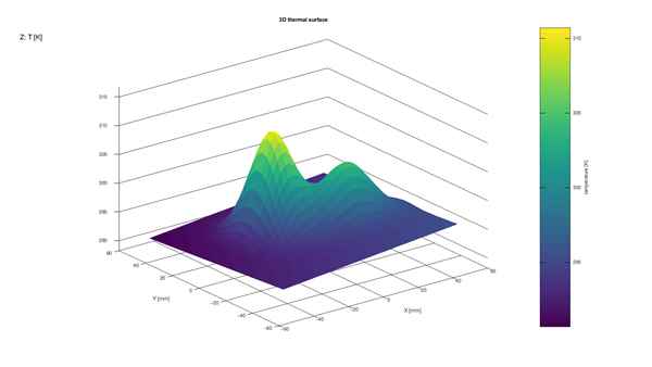
La surface è la vista più intuitiva per comprendere la morfologia complessiva del campo. Il picco principale si trova vicino a X = −12,5 mm e Y = 7,5 mm, esattamente dove lo indica la metrica numerica della Session; il secondo hotspot è più largo e meno intenso.
Questa vista mostra la capacità di GX-TXT di trasformare una griglia XYZ regolare in una superficie scientifica mantenendo unità fisiche sugli assi e sulla colorbar. Il colore non è decorativo: rappresenta la stessa grandezza fisica riportata lungo Z, cioè la temperatura in kelvin.
Perché la superficie appare leggermente deformata?
Azimuth, elevation e projection sono applicati correttamente dal framework: le prove con viste estreme confermano che la camera 3D risponde agli override.
Il difetto osservato resta invece nell'aspect 3D automatico. Nel renderer corrente GX-TXT non impone ancora esplicitamente un daspect/pbaspect coerente. In questo Dataset X e Y coprono entrambi 100 mm e dovrebbero quindi poter essere rappresentati con identica scala visuale; lasciando l'aspect a Octave, il plot box può risultare deformato.
Il problema è di presentazione, non dei valori scientifici del Dataset. Una correzione CORE dovrebbe introdurre un controllo pubblico e persistente dell'aspect 3D, almeno con una modalità equivalente a xy_equal.
2. Mesh: rendere visibile il campionamento
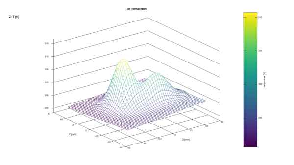
La mesh rinuncia al riempimento continuo della superficie e rende visibile il reticolo sottostante. In questo modo si percepisce immediatamente che il campo non è una funzione analitica disegnata direttamente dal renderer: è una struttura numerica campionata su una griglia regolare.
È particolarmente utile per controllare densità e regolarità del sampling, deformazioni della griglia o eventuali problemi di ordinamento X/Y. Surface e mesh usano lo stesso dato e lo stesso sistema di coordinate, ma rispondono a domande visive diverse.
3. Contour3: isolinee nello spazio
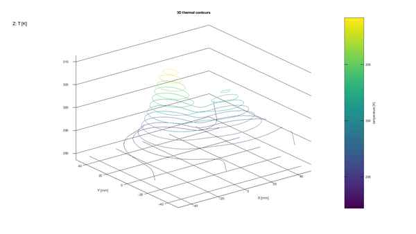
Contour3 elimina la superficie e conserva soltanto livelli discreti del campo. I due hotspot diventano famiglie di curve chiuse: il massimo più stretto produce isolinee più concentrate, mentre il secondo massimo genera strutture più larghe.
Questa vista è utile quando interessa confrontare livelli o soglie piuttosto che osservare una superficie continua. Il numero dei livelli può essere configurato senza modificare i campioni scientifici originari.
Controlli di vista disponibili
La camera può essere modificata da Graphs → Axes... oppure dai Graphics override attraverso Azimuth, Elevation e Projection. Questi controlli funzionano e possono essere verificati con valori estremi, per esempio elevation 90° per una vista dall'alto e 0° per una vista quasi di profilo.
La camera non corregge però l'aspect 3D automatico: cambiare azimuth da −37,5° a −45° modifica realmente il viewpoint ma non elimina la deformazione del plot box.
Tre viste, un solo campo
| Vista | Cosa mette in evidenza | Quando è particolarmente utile |
|---|---|---|
| Surface | Morfologia continua, massimi, minimi e pendenze. | Comprendere rapidamente la forma globale del campo. |
| Mesh | Struttura e densità del campionamento. | Controllare griglia, discretizzazione e ordinamento. |
| Contour3 | Livelli equivalenti della grandezza Z. | Confrontare soglie, livelli e topologia dei massimi. |
Le tre rappresentazioni descrivono lo stesso campo scientifico con finalità differenti. Il Dataset rimane lo stesso; cambia la Plot Variant e quindi il modo in cui l'informazione viene presentata.
Plot.dataset e persistenza
Nella Session HTML eseguita i tre PNG prodotti dal plugin compaiono anche sotto le rispettive Variant plot.dataset.xyz. I checksum coincidono: la copia del plugin e quella della Variant rappresentano lo stesso render.
Surface, Mesh e Contour3 non sono quindi semplicemente immagini isolate. GX-TXT conserva anche configurazione del grafico, fingerprint delle sorgenti, runtime e render cache. La Variant può essere riaperta, modificata ed esportata nuovamente senza trasformare il PNG nel dato autorevole.
Capacità illustrate
- visualizzazione surface, mesh e contour3 dello stesso Dataset;
- binding esplicito X/Y/Z attraverso Variable ID;
- assi e colorbar con unità scientifiche;
- validazione della griglia rettangolare prima del rendering;
- metriche numeriche indipendenti dalla rappresentazione grafica;
- Plot Variant persistenti e rerenderizzabili;
- render cache separata dal dato scientifico;
- nessuna necessità di ripubblicare il Dataset per cambiare tipo di visualizzazione.
Provenienza dei render
I tre render provengono dalla Session surface3d-example, esportata il 26 settembre 2026 con GX-TXT 0.9.8.07. Il plugin documentato è demo.visualization.surface3d 1.0.3 nella baseline GX-TXT 0.9.8.10-dev-031.
Per continuare
- Scientific Dataset Plot — configurazione e persistenza dei grafici 2D/3D.
- Dataset e Variable ID — identità delle variabili X, Y e Z.
- Ticino Valley 3D Cartography Demo — esempio 3D più articolato con layer geografici e campi scalari.
Manuale tecnico completo del plugin
3D Surface Visualization Demo — Manual
Purpose
demo.visualization.surface3d is a deliberately small
GX-TXT demonstration of the framework’s existing 3D scientific plotting
path. It is not a general mathematical plotting module. Its intended
workflow is a finite rectangular scientific Dataset followed by
framework-native surface, mesh, and
contour3 rendering.
The default generated Dataset contains only 41 × 41 = 1681 points so that rendering, rerendering, viewpoint changes, color changes, and regression testing remain practical. Large time-frequency results are intentionally outside the scope of this demo.
Framework and installation
The plugin requires GX-TXT 0.9.7.77 or later.
Install the current demo.visualization.surface3d plugin
package through the normal Plugin Install interface. The plugin remains
external (core=0) and does not modify the framework
distribution.
The deterministic Session Generator is supplied separately as
surface3d_thermal_field_1.0.0.zip and is also bundled
inside the plugin under bundled/. Open the Session
Generator Library Manager, select GX-TXT Numerical
Examples, choose Import Generator…, and import
that ZIP.
Synthetic thermal model
The generator creates a steady-state temperature field over a rectangular plate:
T(x,y) = 293.15
       + 18*exp(-((x+12)^2/(2*9^2) + (y-8)^2/(2*12^2)))
       + 11*exp(-((x-16)^2/(2*14^2) + (y+10)^2/(2*8^2)))
       + 0.03*x
       - 0.02*y
x and y are millimetres and T
is kelvin. There is no random noise.
The coordinate ranges are:
X = -50 mm ... +50 mm
Y = -50 mm ... +50 mm
with 41 positions per axis and 2.5 mm spacing. The complete grid contains 1681 points, ordered with Y as the outer loop and X as the inner loop.
Generated Session files
The generator creates:
raw/thermal_surface_3d.csv
metadata/thermal_surface_3d.metadata.txt
reference/thermal_surface_truth.txt
GX-TXT also writes normal Session Generator provenance to
metadata/session_generator.ini.
The CSV columns are:
x_mm
y_mm
temperature_K
The metadata file uses Dataset Metadata API v1 portable import
syntax. The first = separates key from value, therefore the
analytical equation can itself contain additional =
characters without ambiguity.
The reference truth file exists only for deterministic validation. The normal plugin never reads it.
Recommended import workflow
- Generate a Session with GX-TXT Numerical Examples →
Visualization → 3D Thermal Surface. The suggested Session name
is
surface3d-demo. - Import
raw/thermal_surface_3d.csvwith the normal generic CSV acquisition path. - Open Variables and verify/save the canonical Variable Schema.
- Assign the coordinate quantities as numeric variables with units
mm; assign temperature unitK. The X/Y coordinate variables should have the normal independent-coordinate semantic role and temperature should be measured data. - Open Metadata… → Import…, select
metadata/thermal_surface_3d.metadata.txt, review the fields, and select Save. - Enable 3D Surface Visualization Demo in Analysis.
- Select the imported Dataset as the primary Analysis Source.
- Bind X coordinate, Y coordinate, and Z value to the stable Dataset variable IDs corresponding to X, Y, and temperature.
- Run the module.
Canonical variable IDs, not CSV headers, are the persisted technical identities used by Analysis Source bindings.
Rectangular-grid requirements
Before plotting, the plugin reads only the three selected variables through Table Stream API v3 and verifies:
- X has more than one unique coordinate;
- Y has more than one unique coordinate;
- all X/Y pairs are unique;
- row count is exactly
unique(X) × unique(Y); - every expected grid cell exists;
- X, Y, and Z are finite;
- coordinates can be resolved deterministically to ascending X and Y vectors.
The plugin does not interpolate missing points and does not convert scattered XYZ data into a grid. Invalid data produce an explicit diagnostic.
Summary calculations
The plugin uses NUMERIC_API_v1 descriptive statistics
for the Z values and reports:
- point count;
- X grid size;
- Y grid size;
- minimum temperature;
- maximum temperature;
- mean temperature;
- temperature range;
- X/Y coordinate of the maximum temperature.
The outputs are:
surface3d_report.txt
surface3d_metrics.ini
The source Dataset is not duplicated or republished.
Automatic graphs
A normal Run generates three Graph Provider outputs from the same prepared grid.
Surface
Graph ID:
demo.visualization.surface3d.surfaceArtifact:
01_surface.pngThis uses public gxtxt_plot_surface() from Plot 3D API
v2. Temperature is also used as the color quantity. A colorbar is
enabled by default unless a graph-specific/common graphics setting
explicitly overrides it.
Mesh
Graph ID:
demo.visualization.surface3d.meshArtifact:
02_mesh.pngThis uses public gxtxt_plot_mesh() on exactly the same
scientific grid.
3D contour
Graph ID:
demo.visualization.surface3d.contour3Artifact:
03_contour3.pngThis uses public gxtxt_plot_contour3(). The default is
12 contour levels and can be changed through the graph
configuration.
Axes and units
With the generated Dataset and source units, the automatic labels are:
X position [mm]
Y position [mm]
Temperature [K]
The renderer does not manually scale mm or
K. It uses the current Unit/Dimension and graphics
display-unit infrastructure. Compatible presentation-unit changes remain
presentation state; the Dataset is not rewritten.
Color and viewpoint
The module uses the shared GX-TXT graphics settings for:
- colormap;
- colorbar visibility and label;
- color limits;
- azimuth;
- elevation;
- projection where supported;
- axes/grid presentation.
No plugin-private viewpoint or colormap registry exists.
The default viewpoint follows the current GX-TXT graphics configuration. Graph-specific Axes/3D settings override inherited defaults through the normal framework mechanism.
Render Cache and rerender
The first Run validates the grid, calculates statistics, stores only Dataset identity and small validation metadata in the Render Cache API v1 payload, and creates public Plot.dataset 3D variants.
Presentation-only changes such as azimuth, elevation, colormap, colorbar, color limits, axis presentation, or compatible display units use the normal plot window and persistent Plot.dataset variant. Rerender reads the canonical Dataset through the shared bounded 3D preparation path. The scientific validation and statistics are not recalculated when a valid render cache is available.
If the source Dataset fingerprint changes, rerender rejects the stale cache and requires a normal Run.
Manual
plot.dataset.xyz workflow
The demo does not hide the 3D graphics path. The same imported source
Dataset can be plotted manually with the bundled
plot.dataset module:
- Enable Scientific Dataset Plot.
- Select the same Dataset.
- Bind X = the X coordinate variable, Y = the Y coordinate variable, Z = temperature.
- Enable
plot.dataset.xyz. - Choose
surface,mesh, orcontour3as the 3D plot type. - Run or rerender through the normal plotting workflow.
The rectangular-grid requirements are intentionally compatible with
plot.dataset.xyz gridded rendering.
Expected deterministic reference values
For the default 41 × 41 generator, the reference values are approximately:
point count       = 1681
minimum T         = 290.650005297855 K
maximum T         = 310.708246164604 K
mean T            = 295.044889217262 K
maximum location  = X -12.5 mm, Y 7.5 mm
The generator stores higher-precision reference values in
reference/thermal_surface_truth.txt.
Performance observations
The default grid is intentionally small. Rendering time is recorded
only as an observation when the real Octave render test is run; no
fragile timing threshold is used. In the packaging environment used for
release 1.0.2, GNU Octave was unavailable, so actual
surface/mesh/contour3 timing is reported as SKIP rather
than estimated.
Limitations
- rectangular grids only for the automatic surface, mesh, and contour3 demonstration;
- no interpolation of missing cells;
- no scattered-to-grid conversion;
- no volumetric rendering;
- no 3D selection resource;
- projection capabilities depend on the active Octave graphics toolkit;
- the plugin is a visualization demo, not a general field-processing module.
Public GX-TXT APIs used
- Standard Module API v1;
- Analysis Source Map API v1;
- Analysis Source Metadata Runtime Extension v1;
- Analysis Source Dataset Metadata Runtime Extension v1;
- Table Stream API v3;
- NUMERIC_API_v1;
- Graph Provider API v1;
- Scientific Plot Framework API v1;
- Plot 3D API v2;
- Graphics Inheritance API v1;
- Render Cache API v1;
- Unit Selector / Unit-Dimension APIs;
- Dataset Metadata API v1;
- Plugin Install API v1;
- Session Generator Library API v1.
Validation
TEST_RESULTS.md records the exact tests performed for
this release. Generator and package/install tests execute without
Octave. Real Octave grid-validation and PNG rendering tests are included
and are executed when GNU Octave is available; otherwise they are
explicitly SKIP.
Stable variable identity
The Analysis Source selector may display canonical variable names
such as x_mm, y_mm, and
temperature_K. These display/canonical names are not used
as Dataset technical identities. At runtime the plugin resolves every
binding through gxtxt_analysis_source_variable_meta() and
passes the returned stable variable_id to Table Stream API
v3 together with the selected dataset_id. This is required
because imported Datasets commonly use stable IDs such as
v0001 even when their canonical names are human-readable
column names.